Converting absorption coefficients to reflection coefficients

Most available data are unarguably the Sabine or practical absorption coefficient provided by the manufacturers. For the low frequency prediction using DGM, we need to convert them to pressure-based quantities, i.e., surface impedances or reflection coefficients. This is a challenging task because there are infinitely many surface impedance values that correspond to a single absorption coefficient.

Research on such conversions is scare, but the best way to convert the energy-based absorption coefficients to pressure-based quantity is to categorize the absorber of interest first and use proper surface impedance models to match the input absorption coefficient to the most likely surface impedance based on the model. [1-3]. For example, if one knows the surface of interest is a porous type absorber, then uses a surface impedance model of the same type. To name a few, popular porous absorber models include Delany-Bazley, Miki, Komatsu, and Allard-Champoux, and Biot model, see a summary in [4]. Using those models, we can inversely estimate the primary parameter of the model from the measured Sabine, practical, or normal incidence absorption coefficients.

Treble’s material conversion engine the conversion engine identifies which type absorber it is and generates the most likely surface impedance based on the material type inference. Identifying proper boundary conditions is the most challenging step and this conversion/inference is a very unique feature of Treble, as the other room acoustic software does not provide such information. However, we want to point out that for a given absorption coefficient, there are infinitely many combinations of the real part and imaginary part of the surface impedance, so a relatively large uncertainty lies here.

Treble’s material conversion engine will convert the given absorption coefficient to the most likely surface impedance based on the state-of-the-art knowledge. If you create a very unrealistic material (e.g., acoustic meta surfaces), there is a chance that Treble’s material engine may fail to estimate the surface impedance due to a lack of modeling method of such exotic properties.

In short, Treble needs both the surface impedance and sound absorption coefficient as boundary conditions for hybrid simulations, but you can assign the sound absorption coefficient information and Treble's state-of-the-art material engine will do a conversion for you.

Treble's material engine

Calculating absorption coefficients from surface impedances is straightforward, but the other way is not because we have to reconstruct the lost phase information from real-valued absorption coefficinets. Extracting the surface impedance from the absorption coefficient is thus an inverse problem where an objective function $\chi$ needs to be defined and minimized. $\chi$ is defined with

$$\chi = |\hat{\alpha} - \alpha_{input}|^2,$$

where $\hat{\alpha}$ are the random incidence absorption coefficient computed from the surface impedance model estimated. $\alpha_{input}$ is the absorption coefficient from the manufacturers or that you created.

$$\hat{\alpha} = \int_0^{\pi/2}\frac{sin(2\theta)4 \Re(\hat{Z}) cos(\theta)}{|\hat{Z}|^2 cos^2(\theta) + 2\Re(\hat{Z}) cos(\theta) + 1}d\theta$$

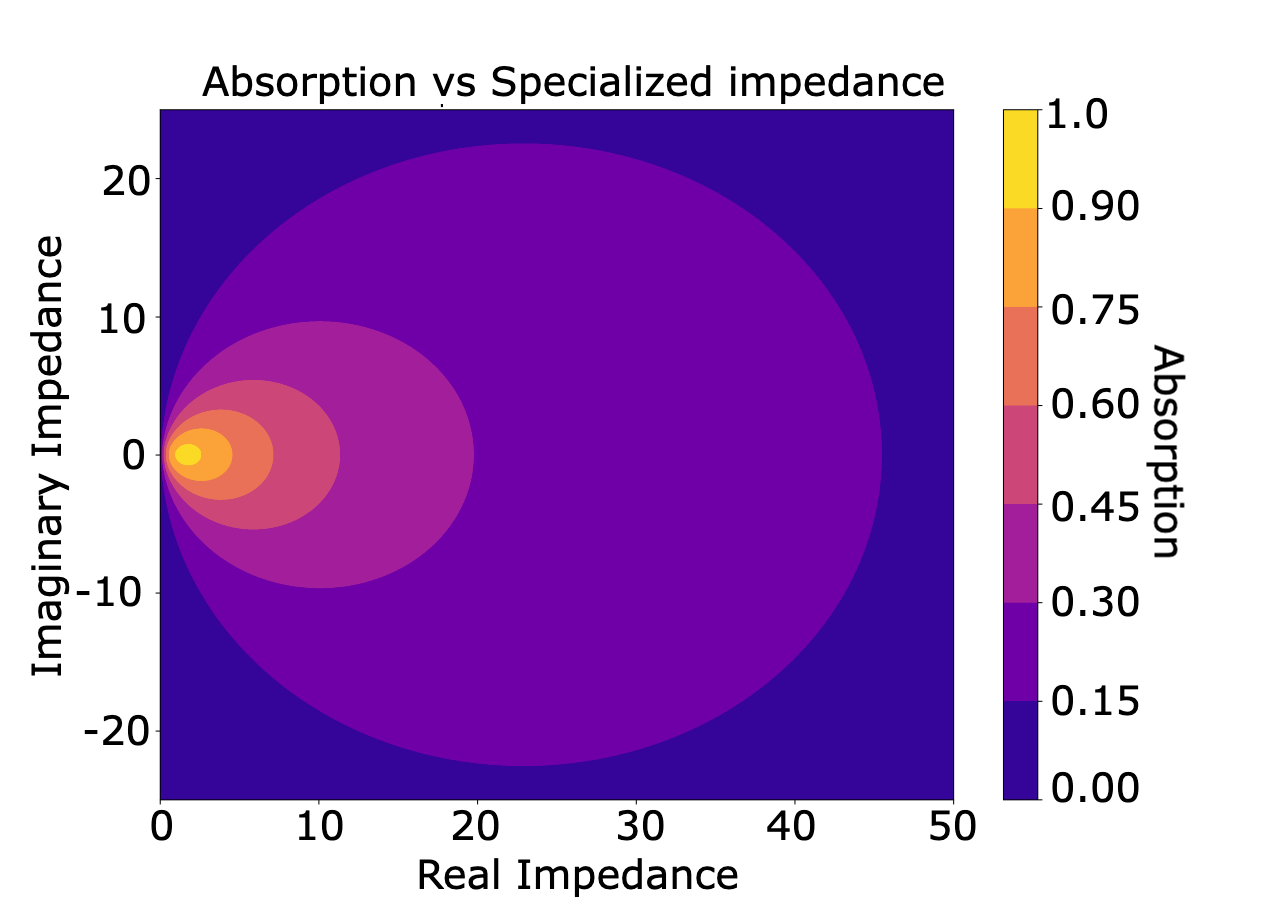
Minimizing $\chi$ is a non-unique problem. The figure here below shows that there are infinitely many combinations of resistances and reactances which explain every absorption coefficient. We thus need to constrain the inverse problem to find what we expect to be a plausible solution e.g. [3].

We further constrain our model depending on the requested level of absorption. In the vast majority of real world cases, materials with low absorption have a larger surface impedance than the chracteristic impedance of air. We thus constrain our model to have normalized surface impedance larger than one for most cases.

Surface impedance to reflection coefficients

As mentioned in the chapter about surface impedance, it is straightforward to compute the reflection coefficient from the surface impedance. Particularly for normal incidence condition, the relation is as follows:

$$R = \frac{\hat{Z}-1}{\hat{Z}+1}.$$

There is yet another inverse process, as the Treble simulation handles the materials with auxiliary differential equations (ADE) at the boundaries of the domain, and those equations need to be posed in a specific way.

Vector fitting

The ADE needs to be represented in a pole-residue model:

$$R^{*}(\omega) = R_{\infty} + \sum^Q_{k=1} \frac{A_k}{\lambda_k + j\omega} + \sum^S_{l=1}(\frac{B_l + jC_l}{\gamma_l + j\beta_l + j\omega} + \frac{B_l - jC_l}{\gamma_l - j\beta_l + j\omega})$$

This process called vector fitting [5-6] is used to find a good direct term ($R_{\infty}$) collection of poles ($\lambda, \gamma, \beta$) and residues ($A, B, C$) to approximate the reflection coefficients as a function of frequency. The vector fitting is another inverse problem where we try to minimize the difference between the true reflection coefficients and the estimated ones. If the input absorption coefficients have a high degree of variability as a function of frequency, it is not guaranteed that the pole residue process will be able to capture the full behavior of the material.

A potential issue with the pole-residue model is that it might result in solutions where $|R| > 1$ and this is non-physical and leads to failures in the simulations (the material is non-passive). This is more likely for rapidly varying absorption coefficients. In case this happens, we take an extra step where passivity is enforced and we minimize,

$$\chi_{pr} = |R^*(\omega) - R^*_{new}(\omega)|,$$

subject to

$$|R^*_{new}(\omega)| < 1 \text{ and } |R_{\infty}| < 1$$

for all values of $\omega$. The final product is then a direct term, $R_{\infty}$, and a collection of poles, $\lambda, \gamma, \beta$, and residues, $A, B, C$, which the Treble simulation engine can understand.

---

References

[1] J. H. Rindel. Modelling the angle-dependent pressure reflection factor. Applied Acoustics.38:223-234, 1993.

[2] C.-H. Jeong. Converting Sabine absorption coefficients to random incidence absorption coefficients. J. Acoust. Soc. Am.,133:3951-3962, 2013.

[3] B. Mondet, J. Brunskog, C.-H. Jeong, J. H. Rindel. From absorption to impedance: Enhancing boundary conditions in room acoustic simulations. Applied Acoustics, 157:106884, 2020.

[4] T. J. Cox, P. D’Antonio. Acoustic Absorbers and Diffusers, Theory, Design and Applications, 2nd ed., Taylor and Francis, 2009.

[5] B. Gustavsen, A. Semlyen. Rational approximation of frequency domain responses by vector fitting. IEEE Transactions on power delivery, 14:1052-1061, 1999.

[6] B. Gustavsen, Improving the pole relocating properties of vector fitting. IEEE Transactions on Power Delivery, 21:1587-1592, 2006.