Modelling the acoustics of a car cabin
Introduction
This case study models the acoustics of a Volkswagen Passat station wagon using the Treble SDK using a wave-based only simulation up to 8 kHz. As for any Treble simulation, we require geometry and boundary condition data to acoustically characterize the cabin. To solve these challenges, we:
- Used a handheld iOS device equipped with LiDAR to capture an initial 3D scan of the cabin's geometry. We refined the scanned mesh using CAD software to produce a watertight, functioning acoustical model.
- Conducted in-situ absorption measurements using a Sonocat probe to establish boundary conditions.
Finally, the model is compared with impulse response data collected through a sine-sweep method.
Special thanks to Dynaudio and DTU for providing access to the vehicle, and Ecophon for lending us their Sonocat device.
Methods
3D Scanning Procedure
We performed 3D scanning using an iPhone 12 Pro, which was manually moved
around the car cabin to capture the car's geometry. The software used to
scan the geometry was the "3D Scanner App" [1],
freely available at the time of writing this article. The app captures the
geometry of the car in .obj format.
As the car interior is compartmentalized, the car doors were open during the scan to allow movement between the trunk, rear, and front. For this reason, the doors were missing from the scan and had to be measured separately.
Next, we imported the scan into FreeCAD 1.0 [2], an open-source 3D modeling software, to trace the geometry of the car's interior. This software uses a non-destructive modeling approach, which is ideal for nuanced geometries such as car cabins. In this process, we simplified the geometry to some extent while making sure larger details, such as the steering wheel, were represented.
Figure 1: Cleaned 3D scanned mesh (in black), with CAD model overlayed (in orange).
We imported the resulting geometry to Rhino via a .step file, where we split
the model into layers corresponding to different boundaries which we assume to
be acoustically homogeneous, and from there we directly import the resulting
.3dm file into the Treble SDK via the geometry import service.
Impulse Response Measurements
We established an evaluation standard by conducting impulse response measurements via exponential sine-sweeps We used a GRAS 46AC 1/2 inch free-field microphone to probe the sound field, which we excite using a small loudspeaker as seen in Figure 2.
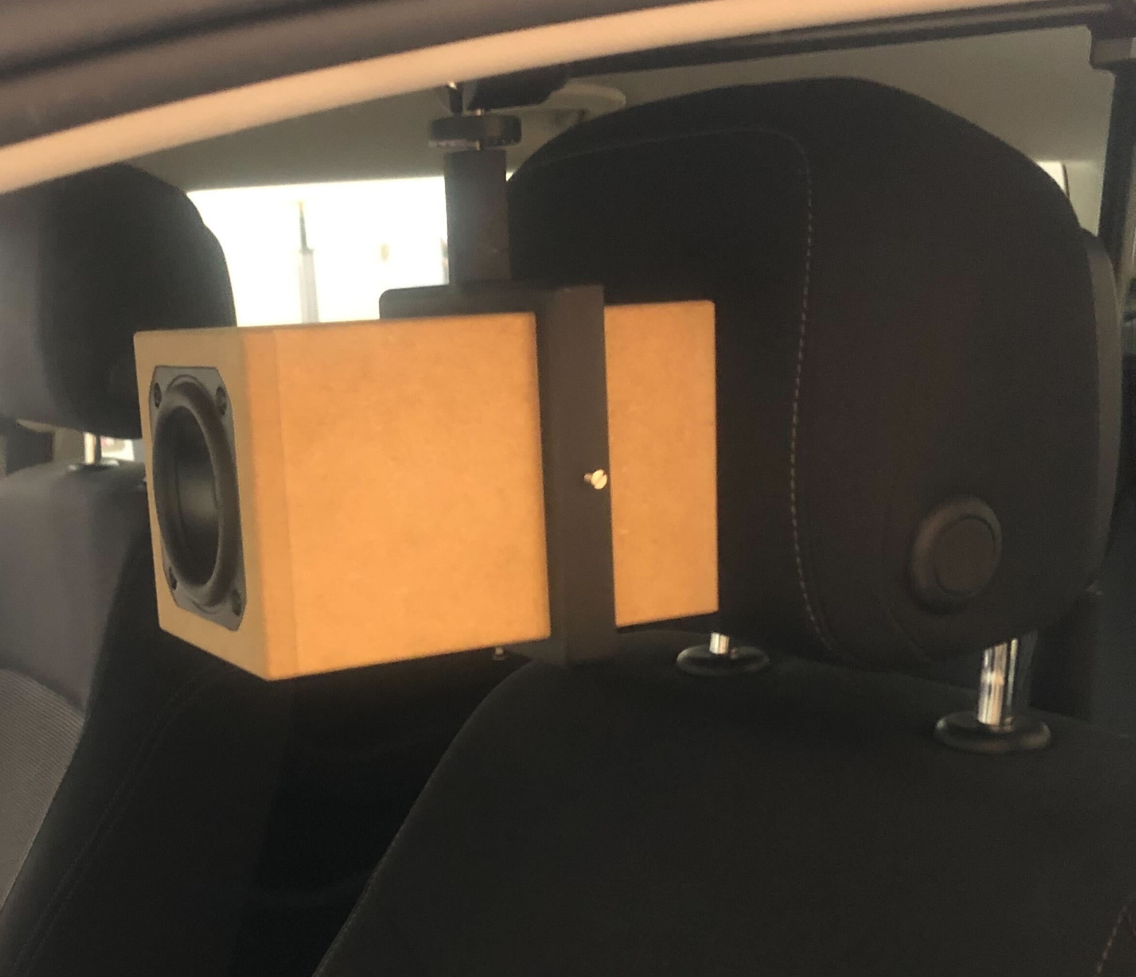
Figure 2: The measurement loudspeaker mounted in the drivers head position.
While this loudspeaker unit was convenient due to its compactness, it has the downside of being unable to reproduce sound below ~115 Hz, as illustrated in Figure 3, which displays estimated SNR spectra in 1/3rd octave bands between 20-8,000 Hz in the measured responses. These estimates are derived by dividing the noise-dominated tail-end of our sine-sweep measurement by the segment populated by the excitation signal, providing a rough estimate of the SNR.

Figure 3: Estimated SNR values are derived by dividing the noise-dominated tail-end of our sine-sweep measurement by the segment populated by the excitation signal, providing a rough estimate of the SNR
Due to the poor signal-to-noise ratio (SNR) at low frequencies, we apply steep high-pass filters to both the measured and simulated impulse responses at 100 Hz to ensure comparability.
Boundary condition acquisition
We conducted in-situ measurements using a Sonocat, a handheld device equipped with a spherical array of eight MEMS microphones and built-in data acquisition hardware. The Sonocat, mounted on a small stand, was positioned approximately 3 cm from each specific surface, ensured by a plastic spacer, while the previously mentioned loudspeaker emitted white noise.
The aim was to align the loudspeaker on-axis with the microphone array and perpendicular to the surface at a maximal distance in order to maximize planar excitation. However, due to the constraining geometry of the cabin, deviations from this procedure were often necessary. Data was recorded via the Sonocat software [3], which automatically processes the data into acoustic properties such as normal impedance and absorption coefficients. A minimum of 3 measurements were done on each layer at varying locations.
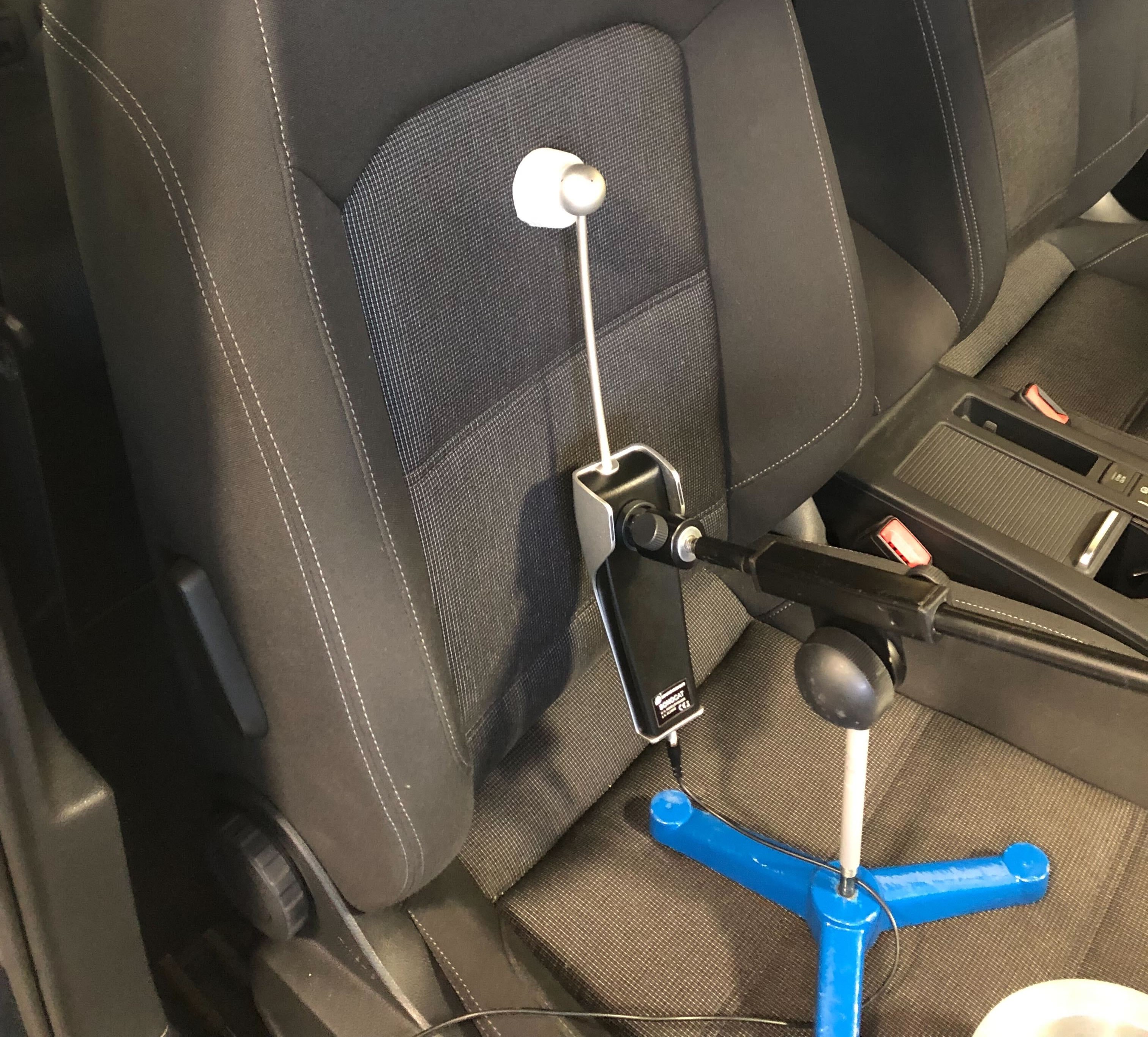
Figure 4: The sonocat was held in position during measurements, and positioned ~3 cm away from the measurement surface, ensured by the white plastic spacer, which was removed during measurements.
Since the time of measurement, we have identified another effective approach, which is using a scanning motion. This method offers clear advantages and is now our preferred strategy. As the measurement setup was available to us for a limited time, we were not able to apply this technique directly during our measurement campaign. Nevertheless, the available data still provided valuable insights. While the yielded impedance estimates proved too noisy for reliable analysis, the absorption coefficients showed consistent trends overall, despite displaying significant variability across measurements of the same layer, with multiple (physically implausible) negative absorption coefficients. To prepare this data for Treble simulations, we averaged results across measurement positions for each layer, excluding any negative absorption values to ensure physically meaningful inputs.
We then explored two approaches for converting these coefficients into Treble materials:
-
Library Matching: Averaged absorption data were compared against all entries in Treble’s material library by computing both the and norms.
-
Spline Smoothing + Treble material fitter: The averaged data was first smoothed using spline fitting, and the resulting curve was passed through Treble’s material fitting engine to obtain the closest match from the library.
We evaluated the outcome of each approach and selected the version that gave the best fit, which in this case was the norm library matching method. Figures 5–7 show example outcomes from each method.
Layer: Passenger front seat cushion

Figure 5: Exploration of material fit candidates for the 'passenger front seat cushion layer', along with the raw and smoothed data averages.
Layer: Dashboard

Figure 6: Exploration of material fit candidates for the 'dashboard' layer, along with the raw and smoothed data averages.
Layer: Front seat headrest

Figure 7: Exploration of material fit candidates for the 'front seat headrest' layer, along with the raw and smoothed data averages.
Simulation and post-processing
To ensure an apples-to-apples comparison between simulations and measurements, two source-related factors need to be accounted for:
- The directivity of the loudspeaker and the simulated source need to match.
- The difference in frequency response between the physical loudspeaker and the simulated source needs to be accounted for.
To help solve both issues, we employ a boundary velocity submodel source in the simulation, which allows us to pre-make boundary velocity sources with specified geometry and inject a them into a simulation. This way, we construct a boundary-velocity submodel of the loudspeaker, approximated by a rigid circular piston representing its membrane and a boxed shape representing its enclosure (see sketch in Figure 8). This way, the directivity of the speaker is largely captured in the simulation, as diffraction effects are inherently modeled in wave-based simulations.
To address frequency response differences, we apply on-axis source correction. Because the boundary velocity submodel sources are calibrated to produce a flat on-axis frequency response of 1 Pa at 1 m in free field, no additional processing is needed in the simulation. For measurements, we perform manual on-axis source compensation at 1 m using Kirkeby deconvolution with an inverse filter derived from an anechoic chamber reference to ensure comparability. The resulting magnitude response is shown in Figure 8 (right).

Figure 8: Schematic of the small loudspeaker used in the project, alongside its measured on-axis magnitude response at an axial distance of 1 meter in an anechoic chamber. The dimensions of the loudspeaker enclosure are (h, w, d) = (100, 100, 160) mm, with a membrane radius of a = 73 mm.
We then placed mono receivers in each seated head position of the cabin, with two extra positions in the luggage compartment. The simulation definition is shown in Figure 9.
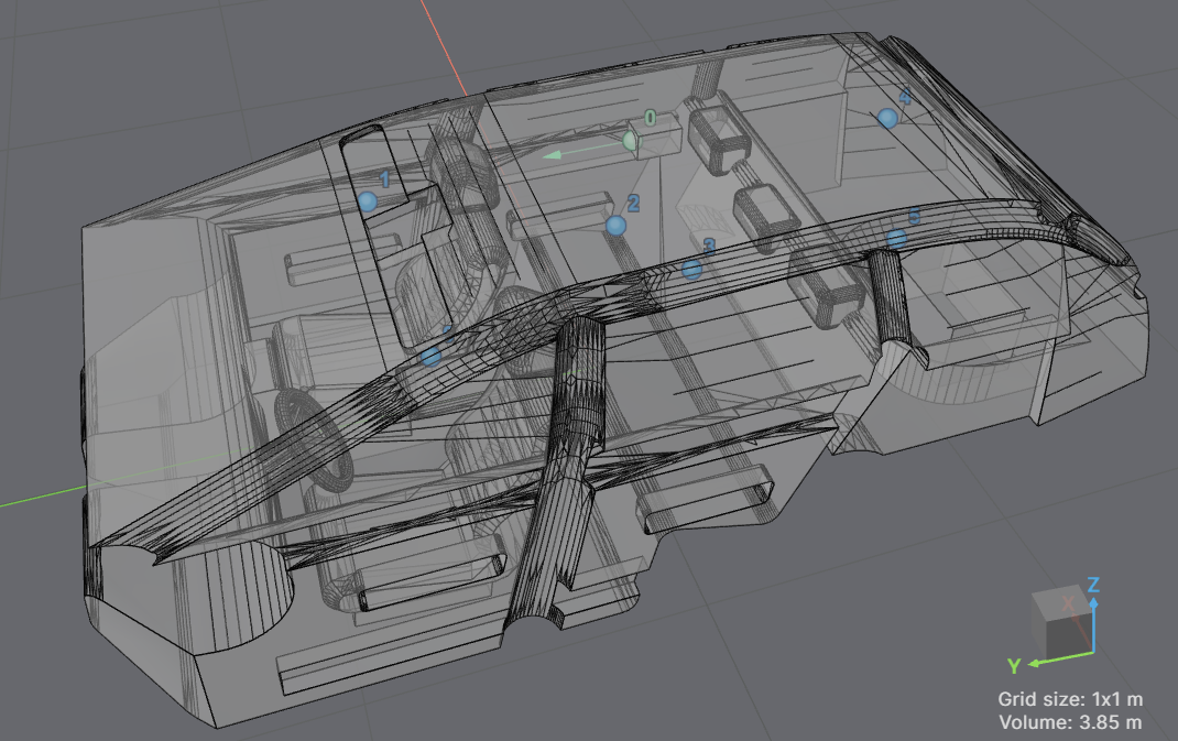
Figure 9: Final cabin geometry visualized via the Treble SDK, along with sources and receivers.
Results
Figures 10 and 11 compare measured and simulated source‑corrected impulse responses and magnitude responses with receiver locations at the driver's head position and the luggage compartment, respectively.
We see that the simulation approximately matches the main peaks and the overall decay envelope in the time domain. However, many large early reflection peaks are missed or slightly shifted. In the frequency domain, the simulation shows reasonable agreement with measurements above 1 kHz, capturing the general spectral slope and multiple resonances. However, most of the narrow-band behavior remains unmatched across the whole spectrum at both receiver positions, especially noticeable low frequencies.

Figure 10: Source-corrected impulse response and magnitude response from source (rear passenger side) to receiver (driver's seat).

Figure 11: Source-corrected impulse response and magnitude response from source (rear passenger side) to receiver (luggage compartment passenger side).
Conclusion
We conducted a fully wave-based simulation of a car cabin using Treble, based on a 3D scan of the interior. The project aimed to explore the feasibility and accuracy of such simulations for modeling in-vehicle acoustics. Our findings suggest that while wave-based methods can provide valuable insights, their accuracy depends heavily on how boundary conditions are represented.
Acquiring reliable boundary condition data was challenging due to significant noise in our in-situ acoustic impedance measurements, likely caused by operator error. As a result, we had to rely on noisy (and non-complex) absorption coefficient data. Improving the measurement method to preserve phase information would likely enhance simulation accuracy. This especially applies in small enclosures like car interiors, where phase effects extend over a broader frequency range and have a greater impact than in larger spaces.
Furthermore, It is likely, that the common assumption of locally reacting, homogeneous surfaces appears fragile in this context, and may not adequately represent the complex, layered materials and coupled cavities typically found in a vehicle's interior.
While accurately modeling the car’s geometry presented challenges, this task is largely manageable with modern CAD tools. In our case, scanning the car cabin using an iPhone equipped with a LiDAR sensor had some limitations in accuracy and detail. Nonetheless, it provided a useful approximation of the interior geometry, which served as a foundation for the CAD model.
These results suggest that improving impedance measurement techniques and re-evaluating how boundaries are modeled will be key steps toward making wave-based simulations accurate and reliable enough for practical use in automotive design.
References
- 3D Scanner App. https://3Dscannerapp.com/. Accessed 7 Aug. 2025.
- FreeCAD: Your Own 3D Parametric Modeler. https://www.freecad.org/. Accessed 7 Aug. 2025.
- Sonocat Software | Soundinsight. 28 Nov. 2022, https://soundinsight.nl/sonocat-software/.