Optimization of a small room for critical listening using Treble

Study by audics - 14 December 2023

Links to audics: Website - Linkedin

Part 1

1. Abstract

The first part of the case study "Optimizing a small room for critical listening with Treble" presents a detailed validation of the discontinuous Galerkin method, using Treble Technologies' Acoustic Simulation Suite (Treble Technologies, 2023). By employing a dense 25 cm x 25 cm measurement grid at ear level, a comprehensive investigation of room acoustics was conducted in a small studio for voice productions, both through physical measurements and virtual simulations. The study demonstrates the impact of speaker positions, particularly regarding their interaction with boundary surfaces and how this can be planned with the simulation. It compares the mode field from both the simulation and real measurements using heatmaps, showing a significant degree of correlation.

2. Introduction

Post Scriptum Audio is a provider of professional voice productions and audiobooks, handling everything from recording to editing and final mastering for publishers, media professionals, and self-publishers from Nuremberg, Germany (Post Scriptum Audio, 2023). The company is planning to move into a new control room, which is to be optimized for high acoustic standards in line with ITU-R BS.1116.

In small control rooms, the room acoustic design below the Schroeder frequency poses a particular challenge, as room modes and interferences with the boundary surfaces are dominant, and space for effective measures is limited. Traditional methods, without knowing the exact pressure distribution in the room, often require laborious measurement processes in a trial and error approach to determine optimal positions for speakers and acoustic treatments. The cloud-based Acoustic Simulation Suite from Treble Technologies enables a wave-based analysis of the room and its sound field using a special form of the finite element method (FEM), the discontinuous Galerkin method. The first phase of the three-part case study documents the validation of the FEM using a 25 cm x 25 cm grid over the entire base area and illustrates the influence of speaker position on the transfer function.

3. Method

3.1. Room

The room of the new Post Scriptum Audio control room has a volume of 38 m3 and is located on the second floor of a historic old building (see Figure 1). The exterior walls are solid, while the interior walls are mostly made of lightweight construction. The ceiling is divided into three differently designed areas, the exact structure of which, like the laminate flooring, is unknown. Some of the walls are not straight and are uneven. The two wooden box-type windows are each equipped with two inner and outer wings and each with glazing. The external wooden blinds were down during the measurement.

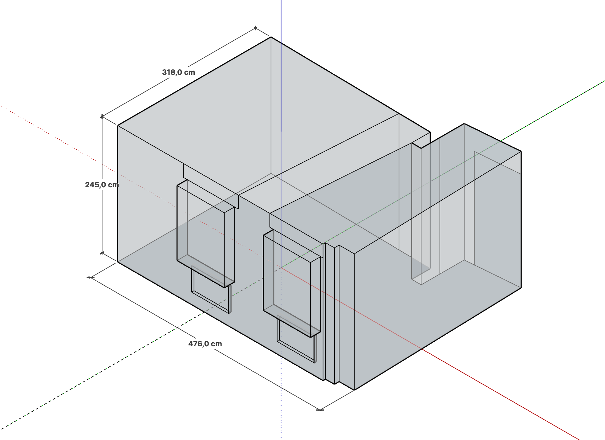
Figure 1 SketchUp model of the empty control room

The Schroeder frequency, which represents the theoretical transition between the modal and diffuse fields, is at 394 Hz, calculated using the formula

$$f_s = 2000 \sqrt{\frac{T}{V}}$$

with T= 1.48 s as the average reverberation time and a volume V of 38 m3. The room eigenfrequencies were calculated for the 3D model on the website of AC Acustica (AC Acustica, 2023) up to 150 Hz and are shown in Figure 2.

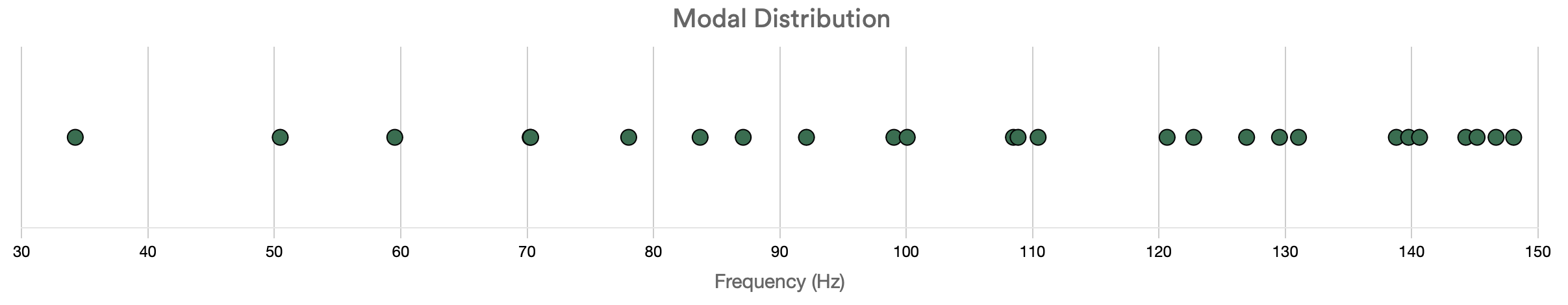
Figure 2 Room eigenfrequencies

3.2 Measurement

The measurement of a total of 229 measurement points was carried out at a height of 117 cm over the entire base area in a grid of 25 x 25 cm (see Figure 3). Along the side walls, the respective measurement row, due to the microphone stand, is 11 cm instead of 25 cm away from the previous row.

The two speakers of the ATC SCM25 A MK2 series were placed on the short side of the room and, together with the measurement position at the listening spot, form an equilateral triangle with a side length of 130 cm. The speakers were measured simultaneously to capture the interaction between them and minimize the measurement effort. Additionally, the left and right sound sources were captured individually along the central longitudinal axis of the room. The mix position is located 176 cm from the front wall, which is about 38% of the room length. The "38% rule" is based on the investigations of the studio designer Wes Lachot (Lachot, 2016), regarding the position in the room where the frequency response in relation to the room eigenfrequencies and low-frequency interferences is most balanced.

The measurement was carried out with the software Room EQ Wizard. An RME Fireface 800 was used as the audio interface and an NTI MA220 Class 1 as the measurement microphone. A logarithmic sine sweep with a length of 11.9 s as the test signal and a loopback as a time reference was used.

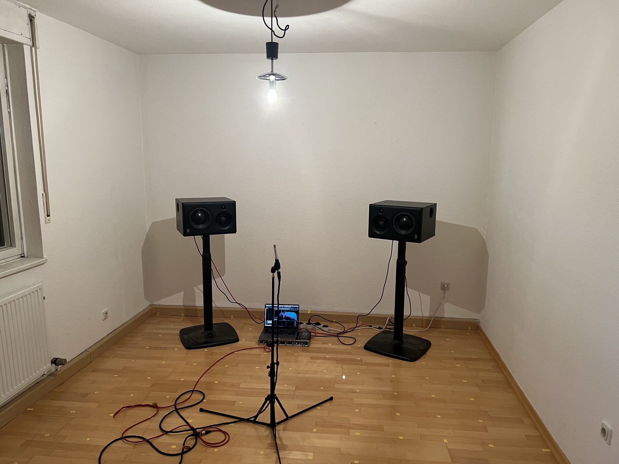
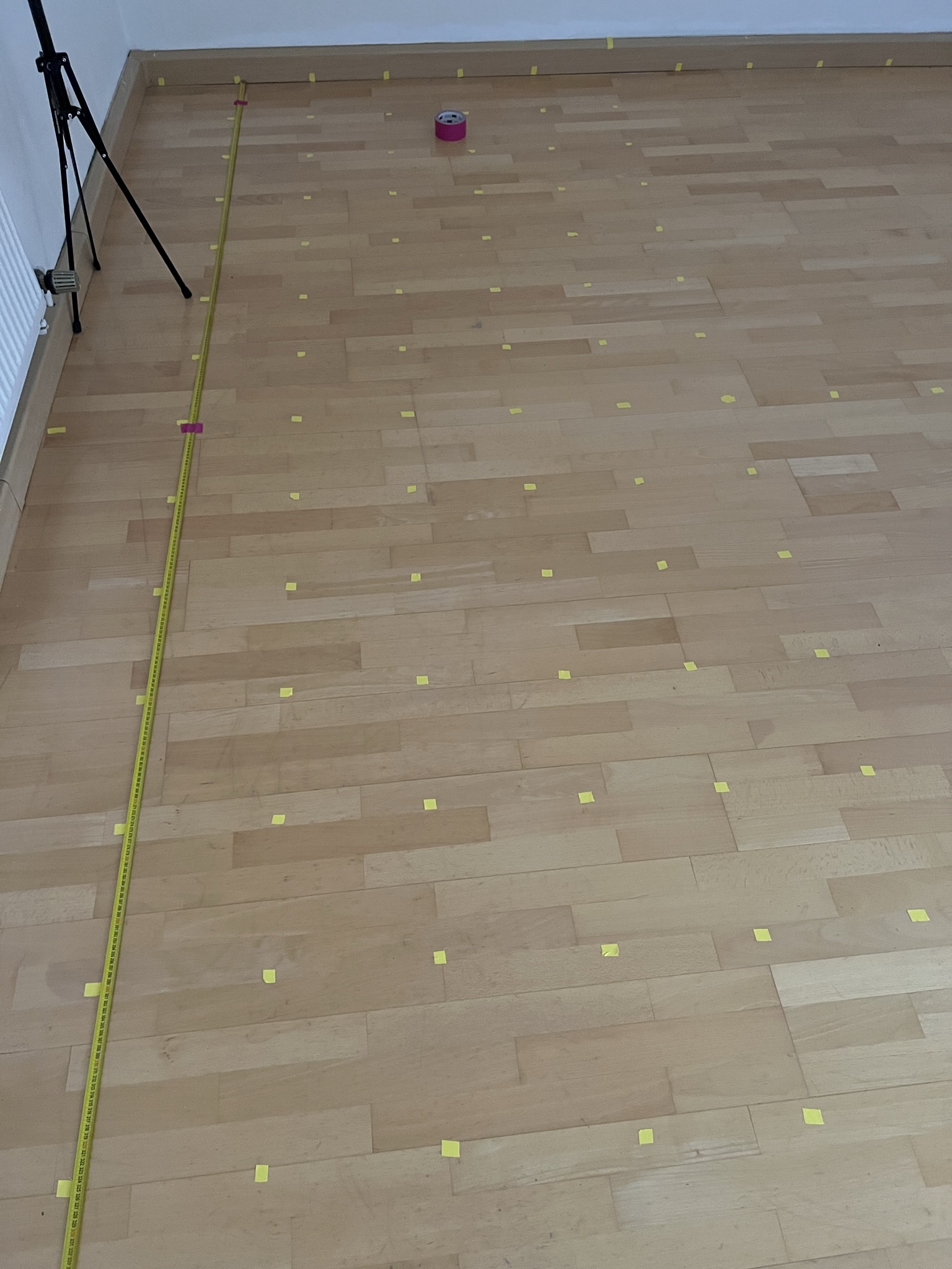
Figure 3 Measurement setup in the real room

3.3. Simulation

3.3.1 Receiver and Sources

201 measurement points were transferred into the simulation (see Figure 4). 28 positions could not be considered due to the distance limitation to sources 1 and 2 and the walls. The origin of coordinates for the 3D model is located at the mix position, here being receiver 108, at floor level.

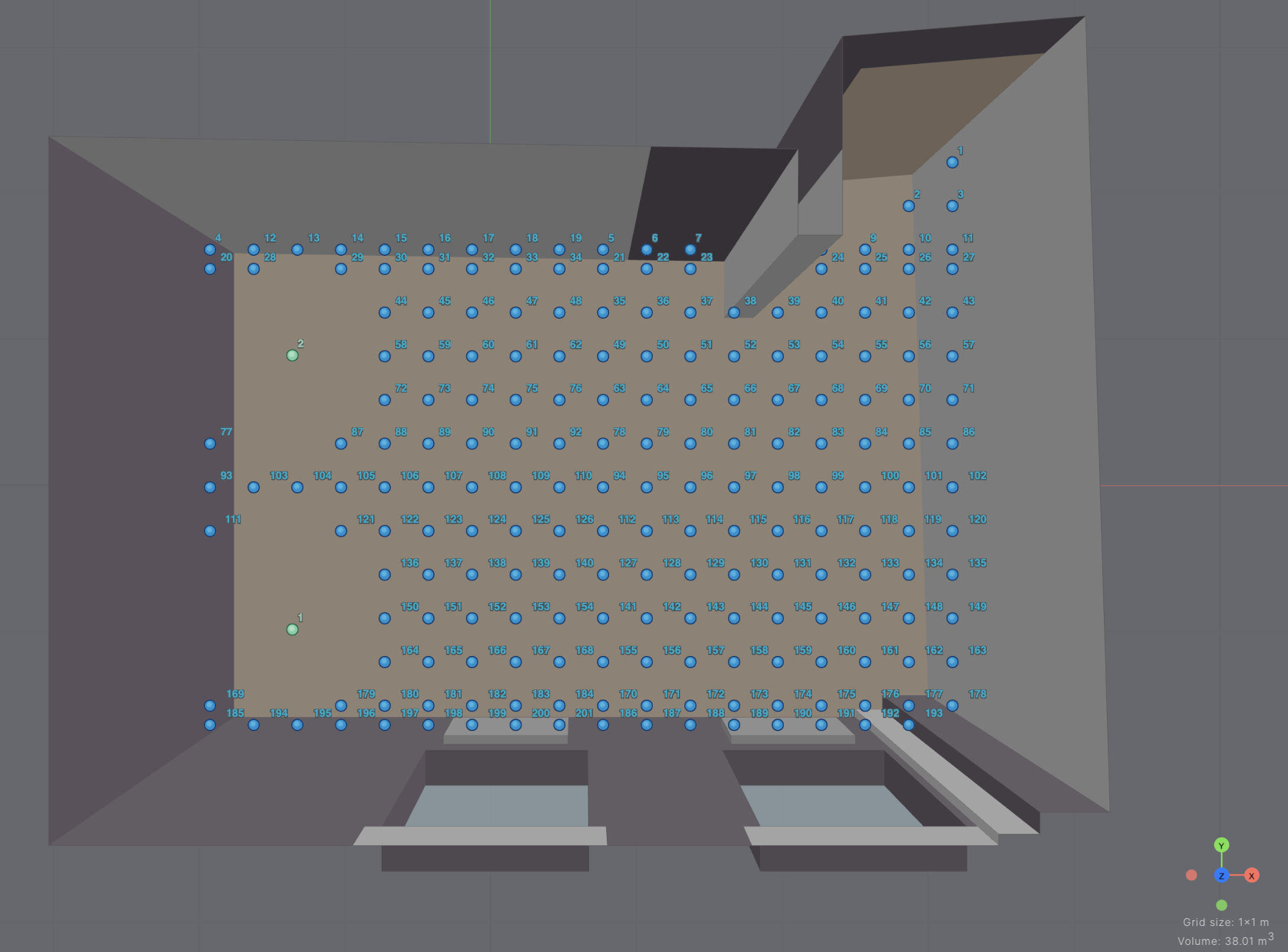
Figure 4 3D model in treble, loudspeaker (green) and receiver (blue), mixingposition (highlighted in yellow)

In the simulation, it is currently not possible to represent the speaker enclosure. Additionally, the directivity and frequency response of the used speakers could not be taken into account, as no data were provided by the manufacturer. Regarding roommodes and interaction with boundary surfaces, the frequency range of 20 – 300 Hz is primarily in focus. Therefore, considering a maximum deviation of +/- 2 dB across the entire frequency spectrum (LoudspeakerTechnologyLtd, 2023), an omnidirectional sound source for the low-frequency driver was chosen as a sufficient approximation.

3.3.2 Speaker Boundary Interference Response

In the first attempt, it was assumed that the acoustic center was located in the middle of the speaker. Up to 100 Hz, the frequency response plots in figure 5 also indicate that this is a valid assumption.

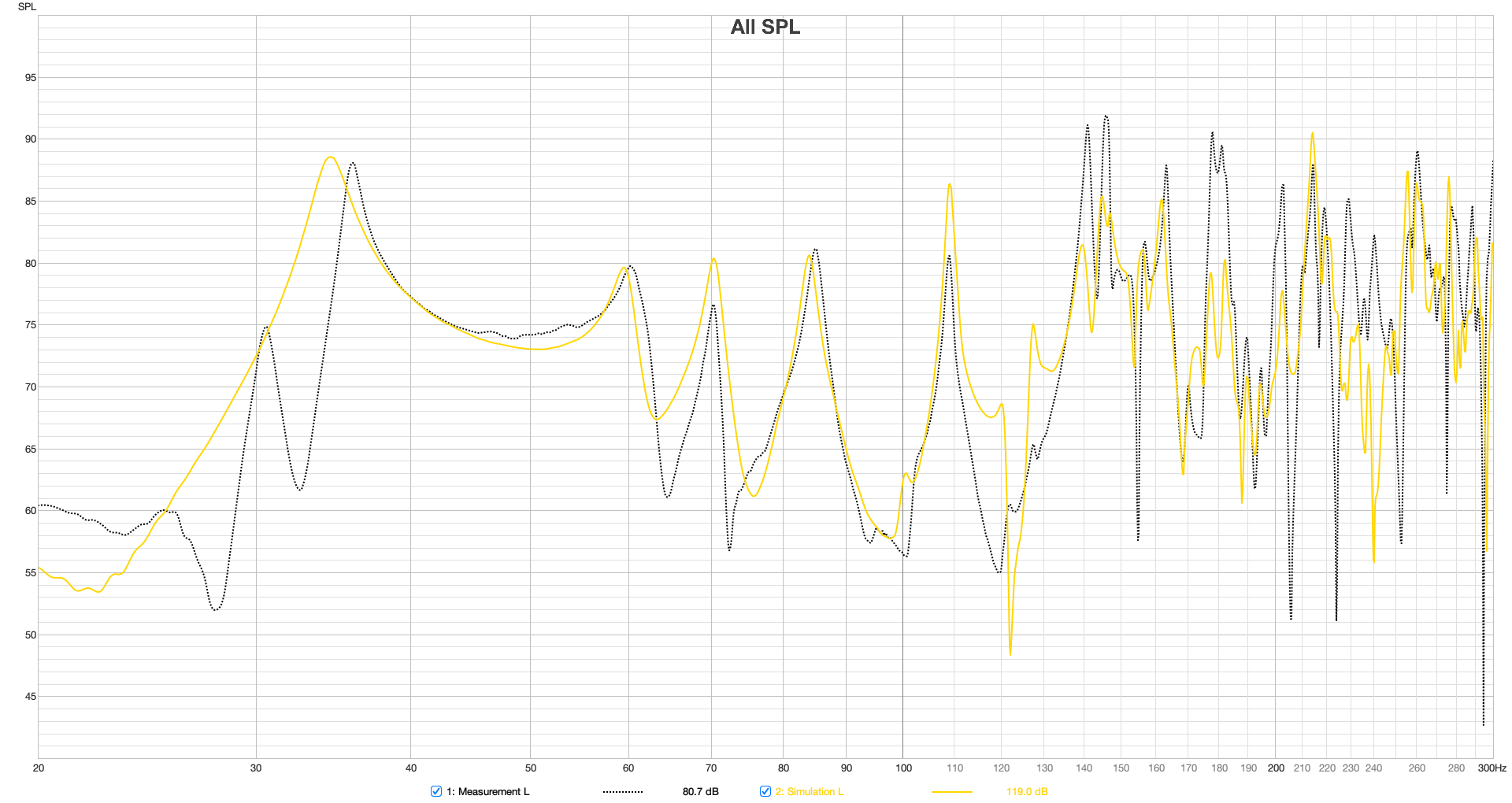
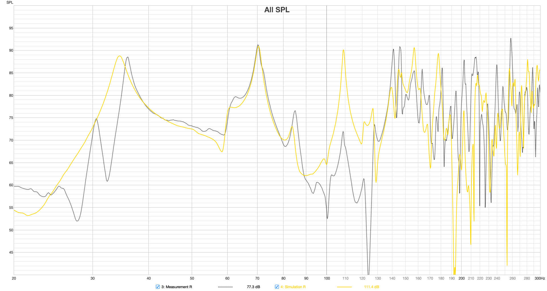
Figure 5 Frequency responses to the left and right of the source position, centered on the speaker enclosures

However, above 100 Hz, the sound propagation from the source is no longer completely spherical due to the speaker enclosures (see the term of Baffle Diffraction (Tripp, 2022)), leading to a divergence in the results from measurement and simulation because of the different path lengths to the boundary surfaces. The acoustic phenomenon observed here is referred to as Speaker Boundary Interference Response (SBIR), responsible for characteristic dips in the frequency response. It results from the destructive interference between direct sound emitted from the speaker and indirect sound reflected off boundary surfaces. When the path length difference between the direct and indirect sound exactly corresponds to half a wavelength, destructive interference of the two wavefronts occurs, resulting in a noticeable dip in the frequency spectrum (Mellor, 2016).

Therefore, the frequency response at the measurement positions is determined by both the room's eigenfrequencies from Figure 2 and the interference with boundary surfaces. Figure 6 shows nine speaker positions arranged in a 10 cm x 10 cm grid.

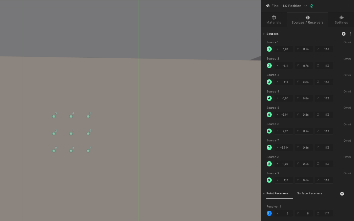
Figure 6 Nine speaker positions arranged in a grid of 10 cm x 10 cm

The significant impact of the position on the frequency response is demonstrated in Figure 7. The peak at 109 Hz, where the second axial mode of the room's width and the third axial mode of its length coincide, varies by up to 26 dB within the displayed arrangement, depending on how it overlaps with interference from the first reflection. The difference between mode and reflection can be recognized by the fact that the frequency of the latter changes with the position, particularly in the 100 - 130 Hz and 170 - 200 Hz range. Due to the wave-based and frequency-accurate analysis with Treble, this phenomenon can for the first time be identified and addressed already in the planning stage using room acoustic simulation software.

Figure 7 Frequency response of the measurement and sources 1 (Simulation_R) to 9 receiver 108

The manufacturer (LoudspeakerTechnologyLtd, 2023) indicates the acoustic center of the speaker as being in the middle of the midrange driver, as shown in Figure 8.

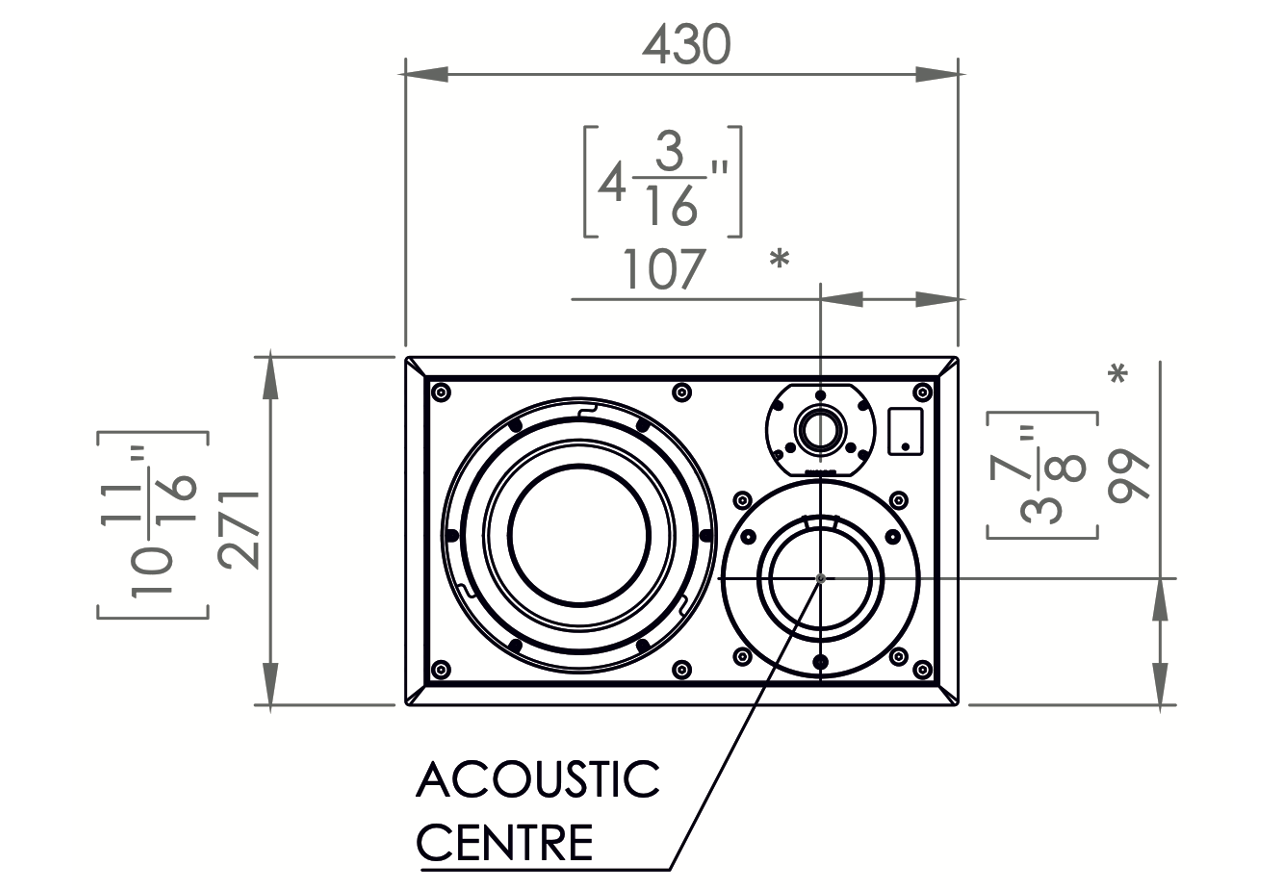
Figure 8 Acoustic center ATC SCM25 A MK2

Due to the approximated modeling of the sound source, the position of the point sound source in the simulation was finally offset, arranged to match as closely as possible with the sound pressure distribution over the entire area as per the measurement (see Figure 9).

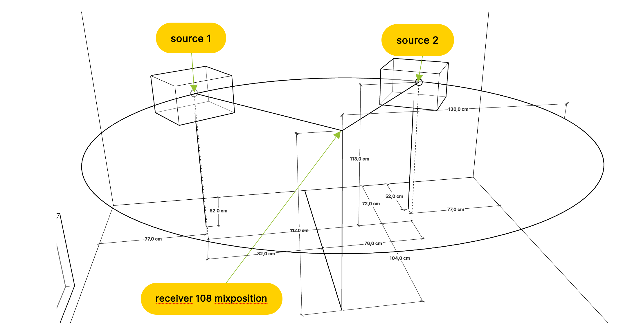
Figure 9 Position of the speakers and the listening position in the simulation

There is a slight offset between the arrival of impulses from the measurement and simulation (see figure 10). On the left, they arrive simultaneously, while on the right, the simulation arrives 0.06 ms earlier. This implies that the right sound source is positioned approximately 2 cm closer to the receiver in the simulation than in the measurement.

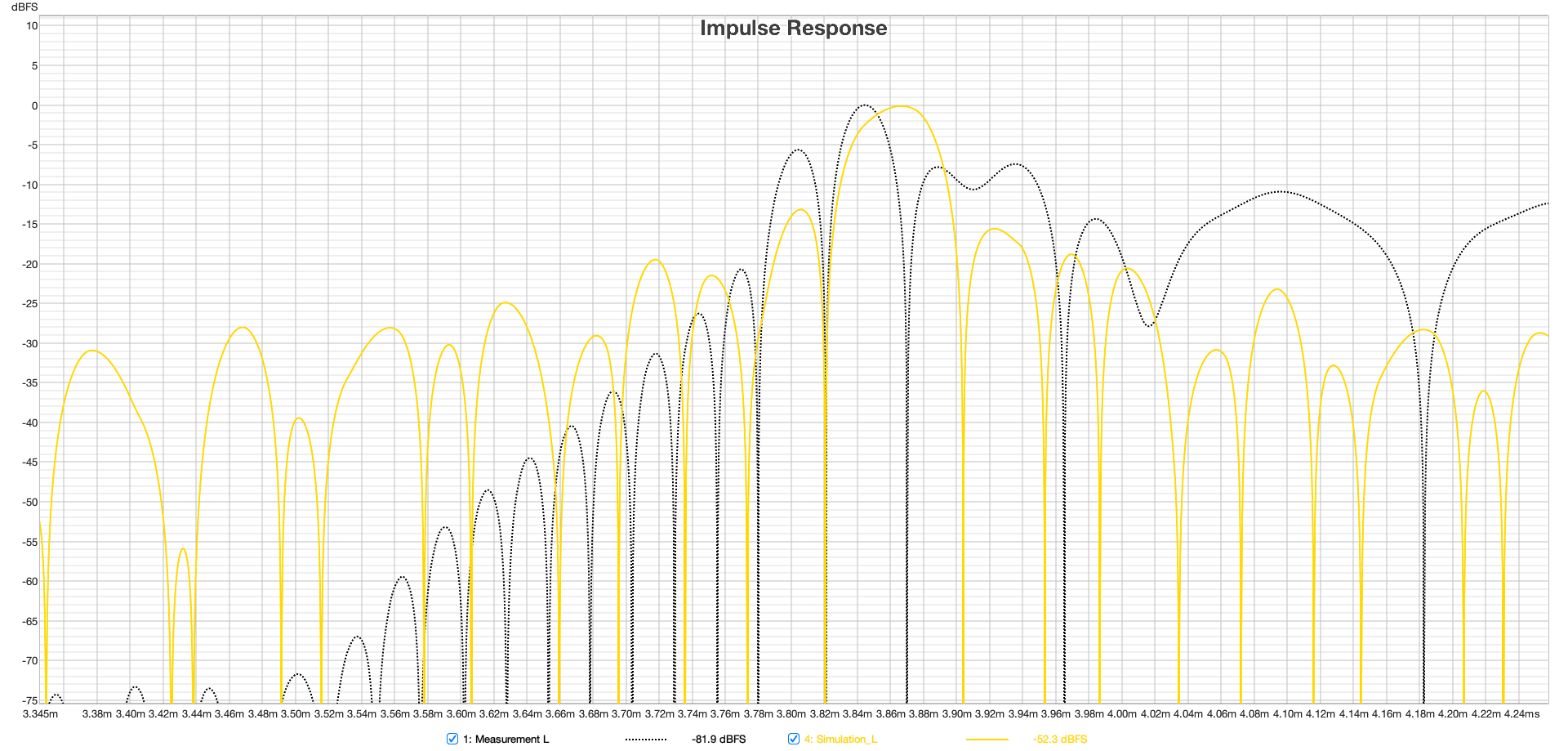
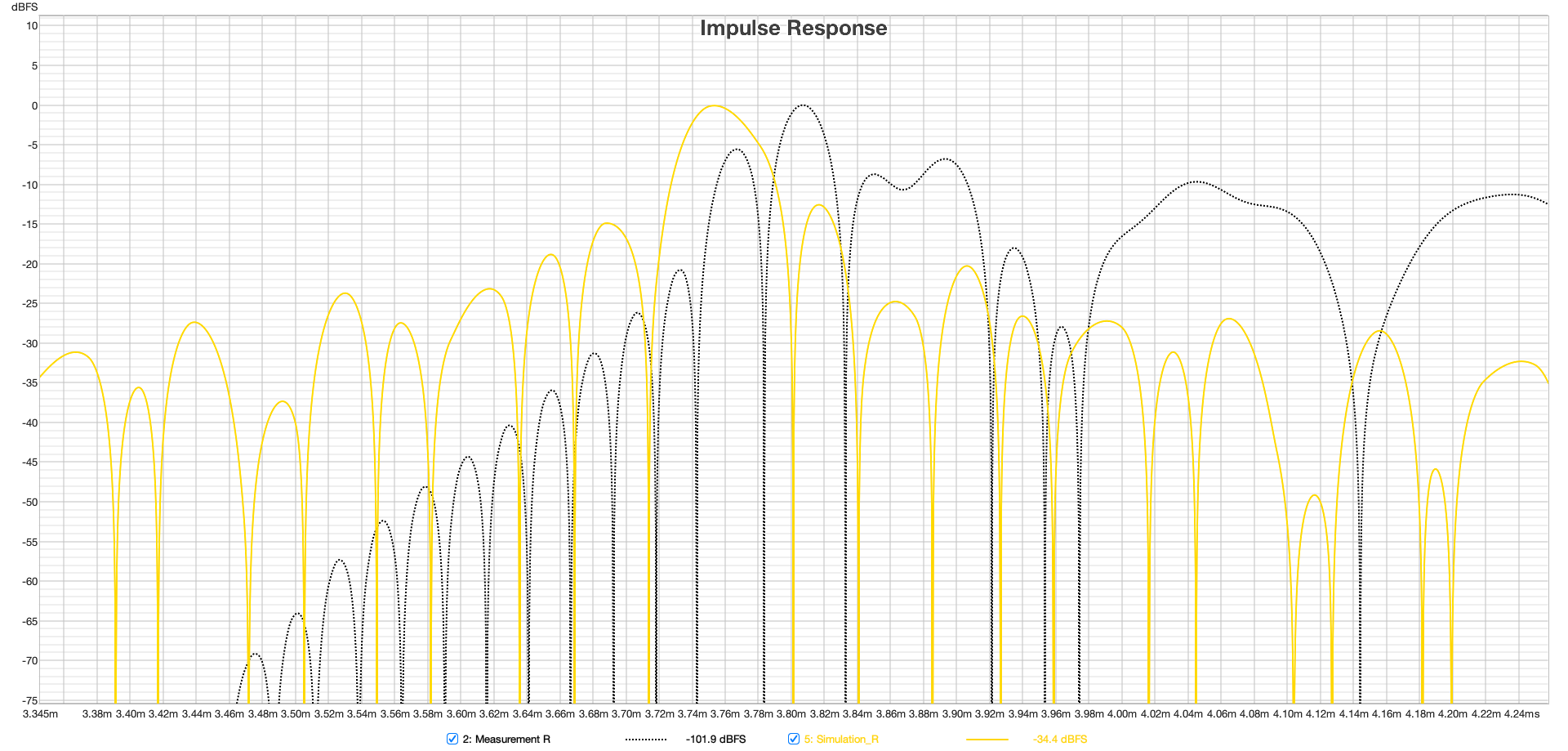
Figure 10 Temporal relationship between the pulses of measurement and simulation, left and right

3.3.3 Absorption coefficients

In the next step, the reverberation time at the mix position in the simulation was adjusted to match the measurement by tuning the absorption coefficients of the surfaces. The Acoustic Simulation Suite from Treble requires both the acoustic impedance of the surface for the wave-based part of the simulation, as well as the reflection coefficient and scattering degree for the geometric part above the transition frequency. Treble's Material Engine offers the possibility to automatically calculate back to impedance and pressure-based reflection coefficient by specifying the diffuse absorption coefficient and material type (Treble technologies, 2023).

Efforts were primarily made to approximate the focused area below 300 Hz as closely as possible to the measurement. This was limited by the fact that the absorption coefficients could only be edited with octave precision in the frequency range starting from 63 Hz. The dip in reverberation time at 500 Hz was attributed to the box windows and the door. The final inputs used are listed in Table 1.

Table 1 Materials and absorption coefficients used in the simulation

Absorption coefficients	63 Hz	125 Hz	250 Hz	500 Hz	1000 Hz	2000 Hz	4000 Hz	8000 Hz
Ceiling old building	0.02	0.02	0.05	0.05	0.05	0.05	0.05	0.05
Ceiling beam	0.06	0.06	0.06	0.06	0.05	0.03	0.03	0.03
Gypsum plasterboard ceiling	0.15	0.12	0.09	0.07	0.05	0.04	0.04	0.05
Solid walls	0.02	0.02	0.03	0.03	0.02	0.01	0.01	0.01
Gypsum plasterboard with mineral wool	0.23	0.12	0.10	0.09	0.06	0.04	0.04	0.06
Gypsum plasterboard without mineral wool	0.09	0.07	0.06	0.05	0.04	0.04	0.05	0.07
Door	0.06	0.06	0.07	0.12	0.08	0.06	0.05	0.05
Heating radiators	0.03	0.03	0.03	0.03	0.03	0.03	0.03	0.03
Box-type windows	0.36	0.35	0.25	0.37	0.08	0.06	0.01	0.01
Floor	0.04	0.04	0.04	0.05	0.06	0.06	0.06	0.06

4 Results

The transition frequency of the simulation between wave-based and geometric calculation for the shown results is set at 3 kHz. This high frequency was chosen to analyze the decay behavior up to and including the midrange with high resolution. The impulse responses have a length of 1.9 s. The computation time for two sources and 201 receivers was approximately 3 hours, plus about 1 hour of software-internal post-processing of the impulse responses. For a transition frequency of 1 kHz and 201 receivers, the computation took 38 minutes, for 1 kHz and one receiver 8 minutes, and for up to the Schroeder frequency of 394 Hz, only 3 minutes were required.

4.1 Decay time

The plots in Figure 11 of EDT, T20, T30, and Ts for both left and right speakers at the mix position show a very good match above the Schroeder frequency between the simulation and measurement.Slight differences in the midrange between 500 and 1000 Hz suggest that the room's damping in this spectrum was slightly underestimated. Particularly noteworthy is the good agreement of the Early Decay Time (EDT), which is often used in assessing room reverberance and is highly location dependent.

The classical RT60 calculation in the time domain is based on the analysis of the Schroeder integration, which sums up the energy of the impulse response in reverse to determine various RT60 values (like T20, T30). However, this method has limitations and is particularly unsuitable for narrowband filtering below the Schroeder frequency. An alternative approach is to calculate reverberation times by analyzing decay times in several steps of a Short-Time Fourier Transform (STFT), here referred to as RT60M (Mulcahy, 2022). This method allows for more precise filtering (see Figure 11). Unlike the time-domain method, each resonance can be individually identified here. The plot shows overall a very good match from 50 Hz up to the transition frequency at 3 kHz. The visible resonances below the Schroeder frequency of 394 Hz dominate the decay times in the classic RT60 plots of Figure 10 in this area. Additionally, the transition between the wave-based and geometric calculation portion is noticeable.

In Figure 13 and Figure 14, the spectrogram of both speakers from measurement and simulation at the mix position over a 60 dB decay is shown. Overall, it is evident that, apart from the decay at 109 Hz and 147 Hz, the temporal behavior of the room in the simulation is captured very well.

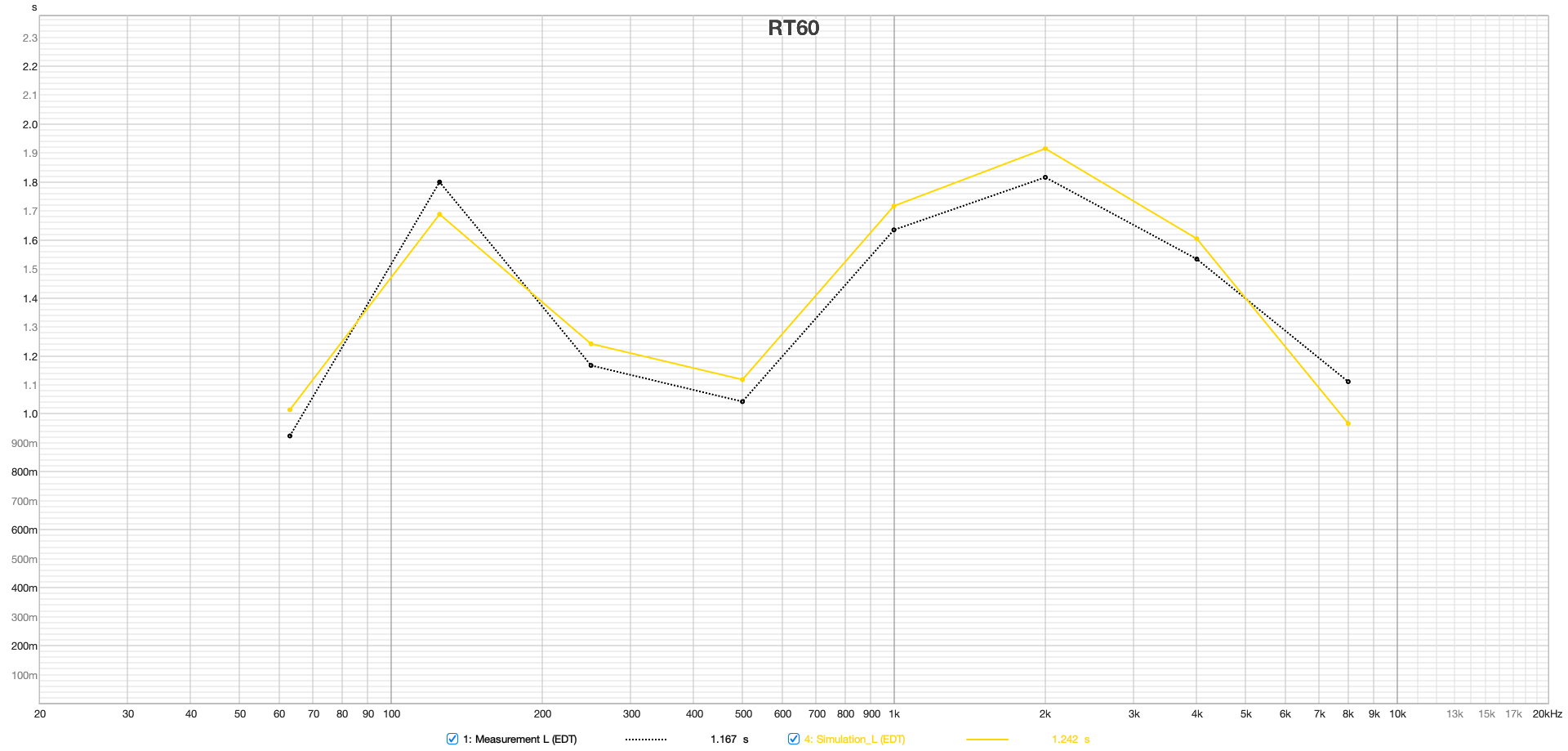
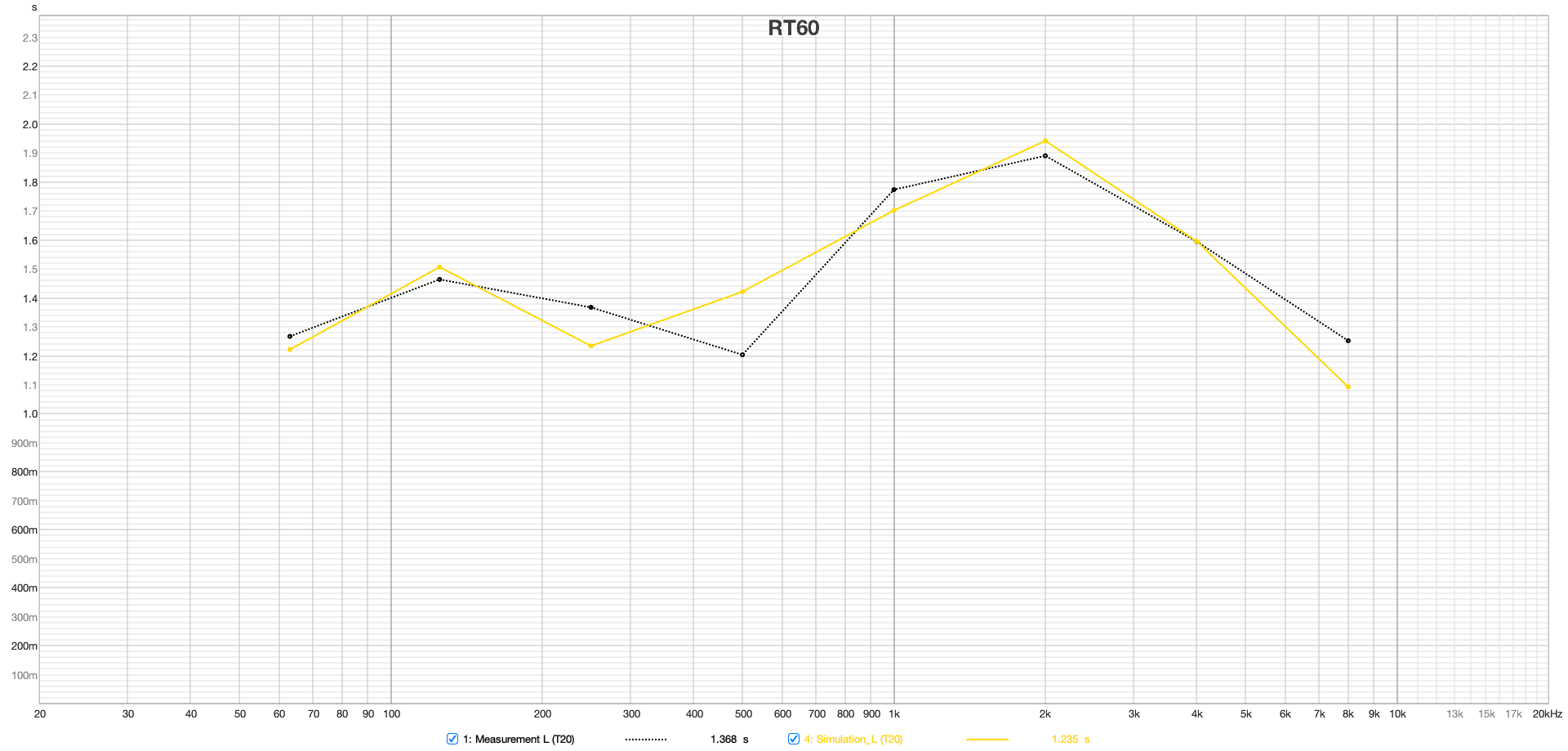
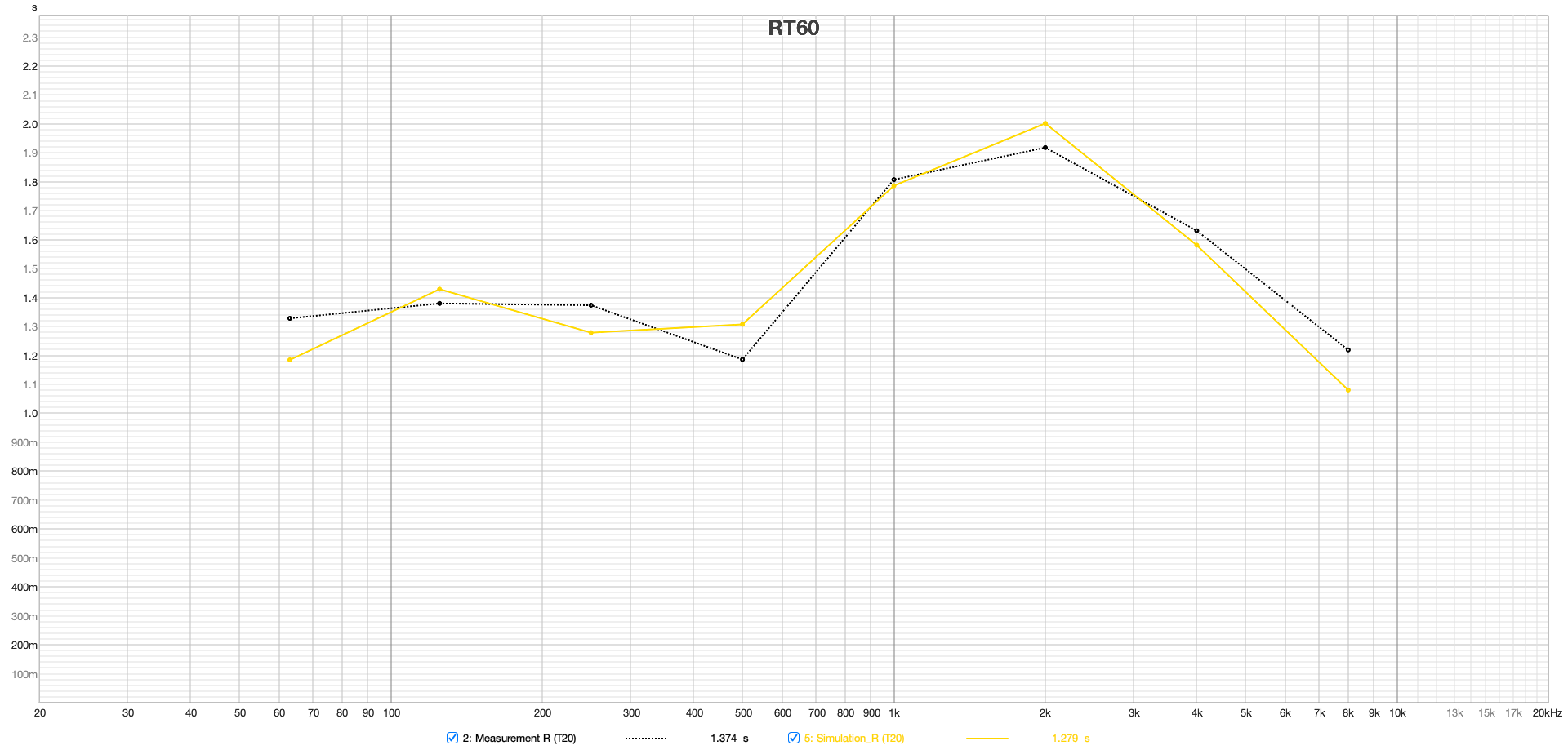
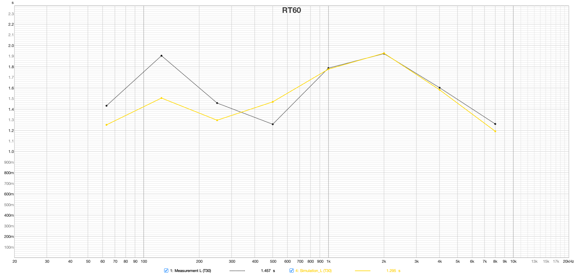
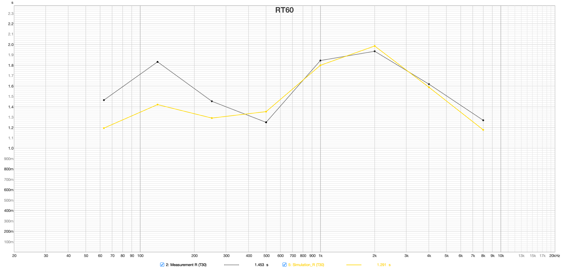
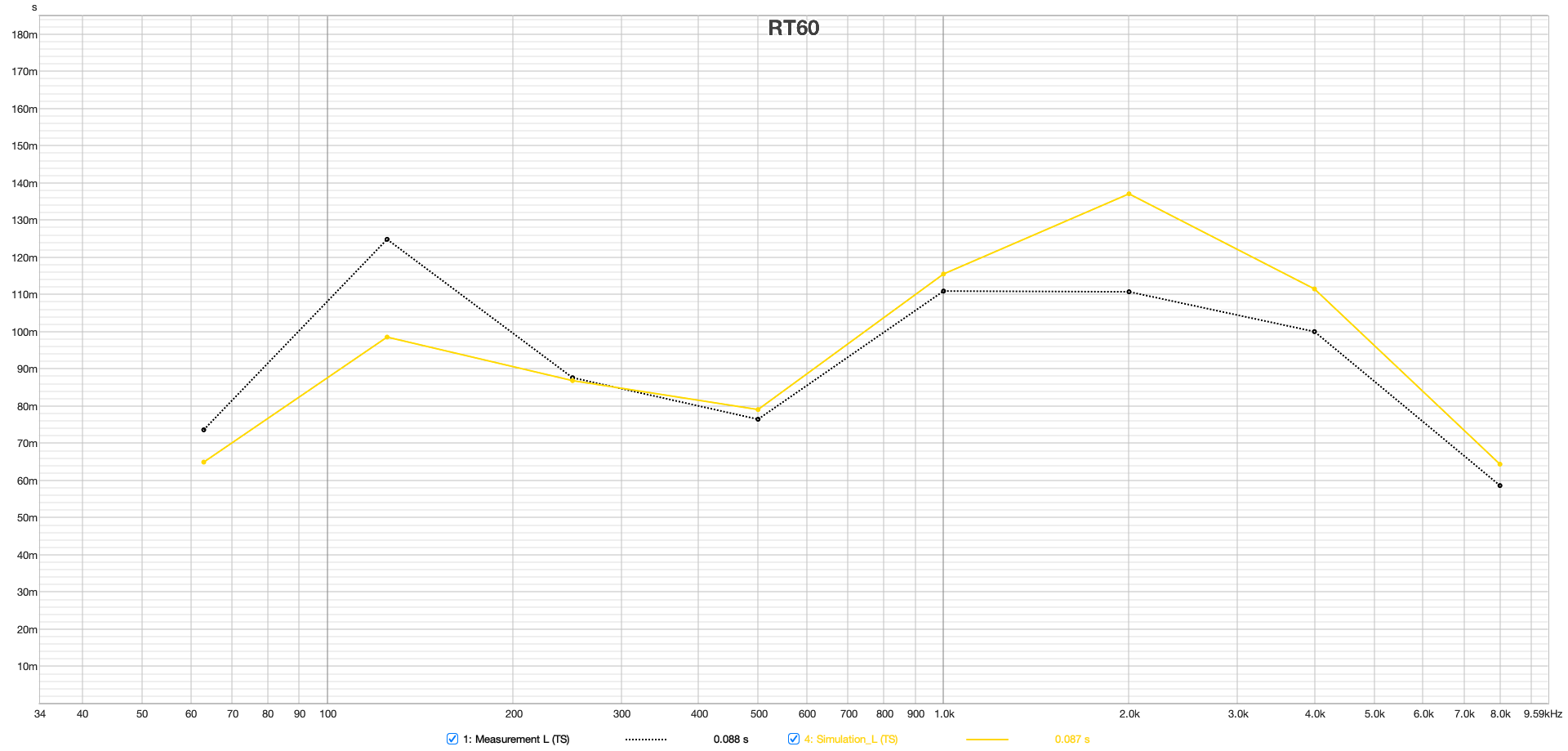
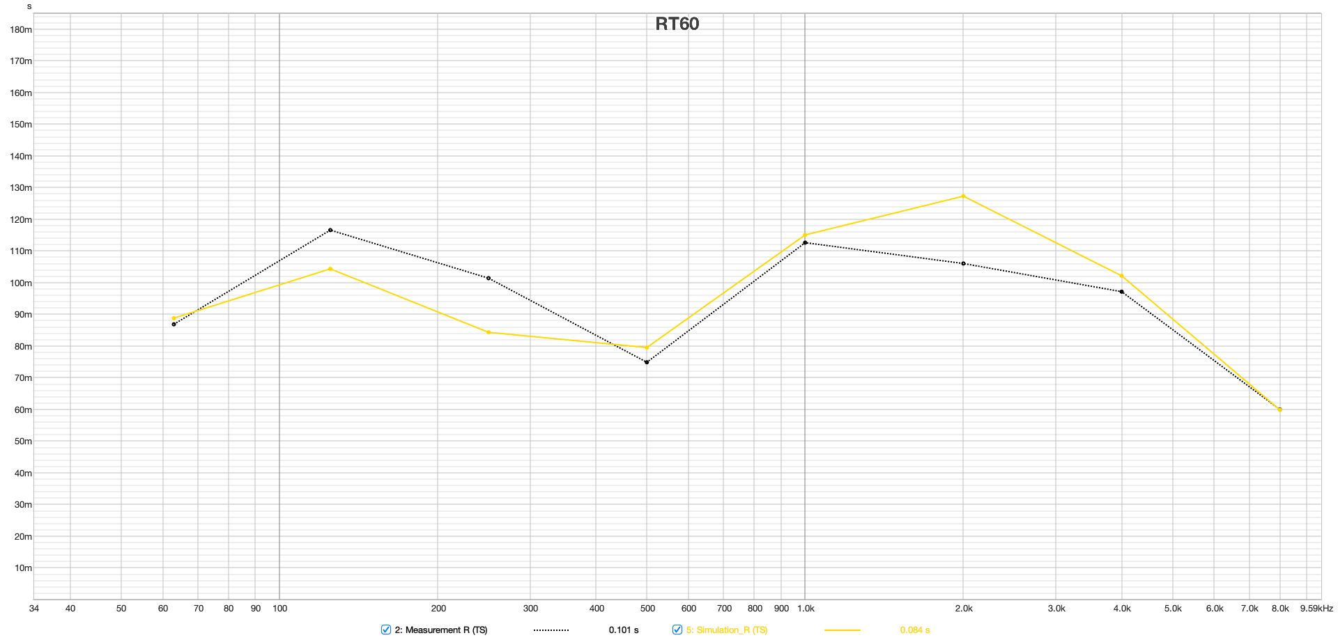
Figure 11 from top to bottom: EDT, T20, T30 and Ts, left and right speakers at the listening position

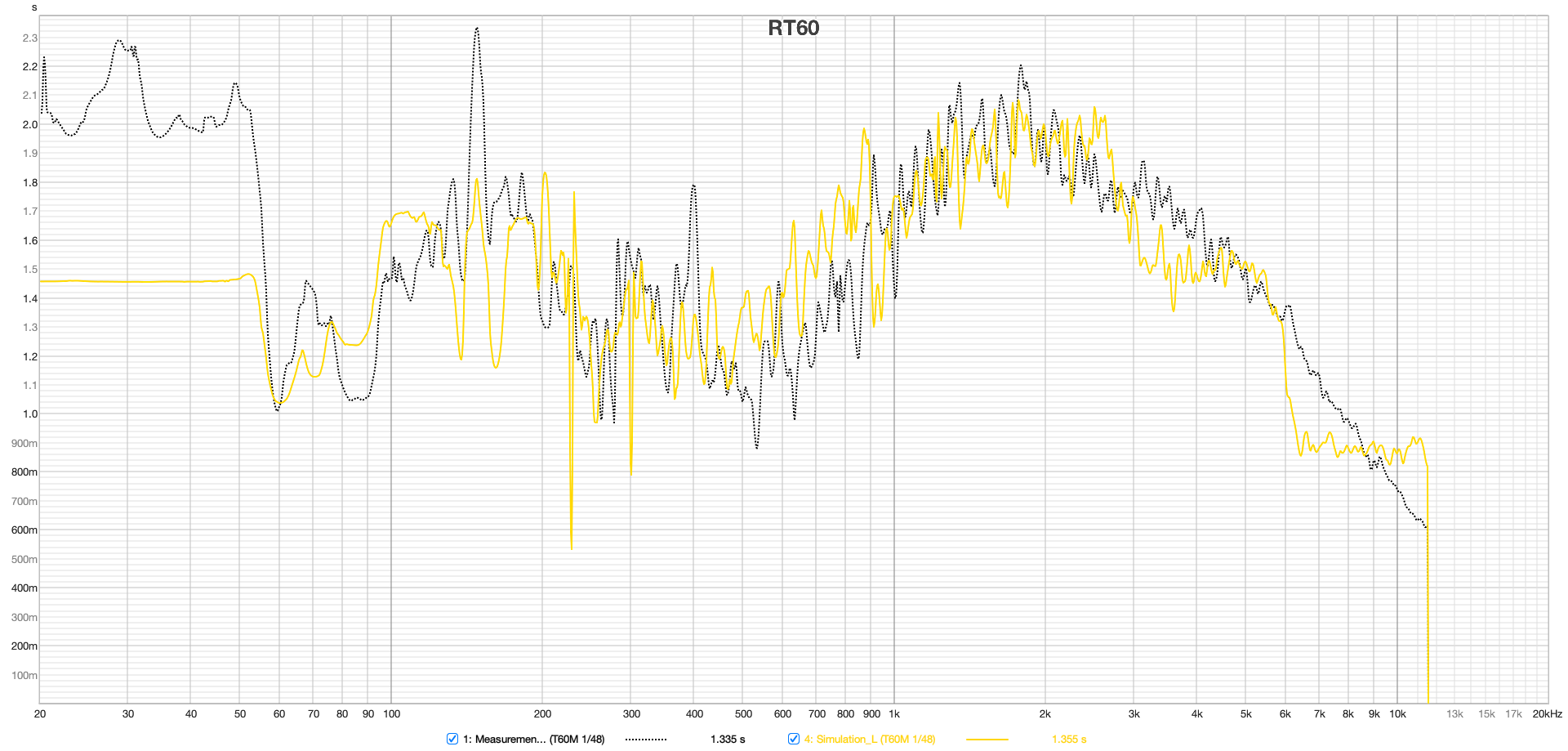
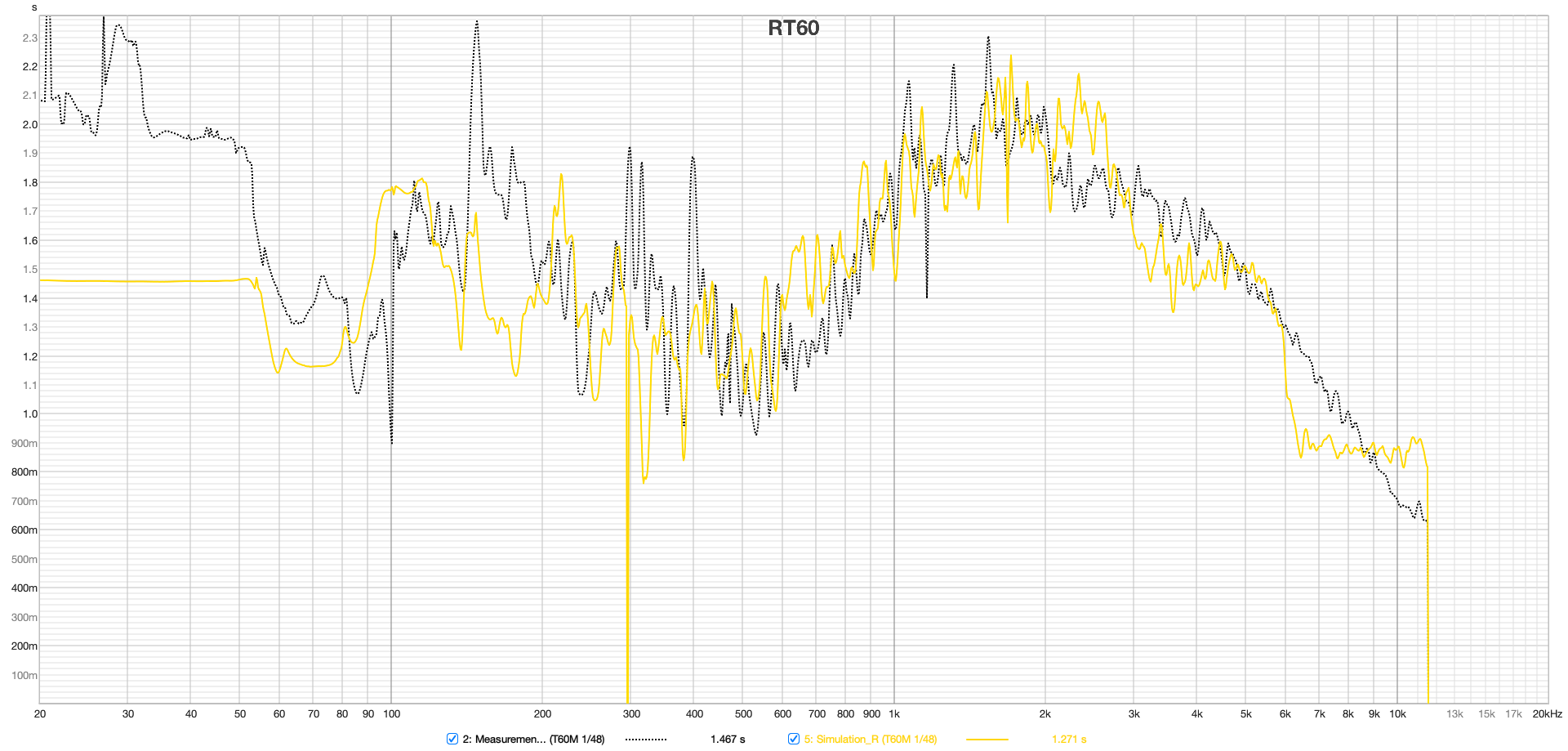
Figure 12 RT60M, left and right speakers at the listening position

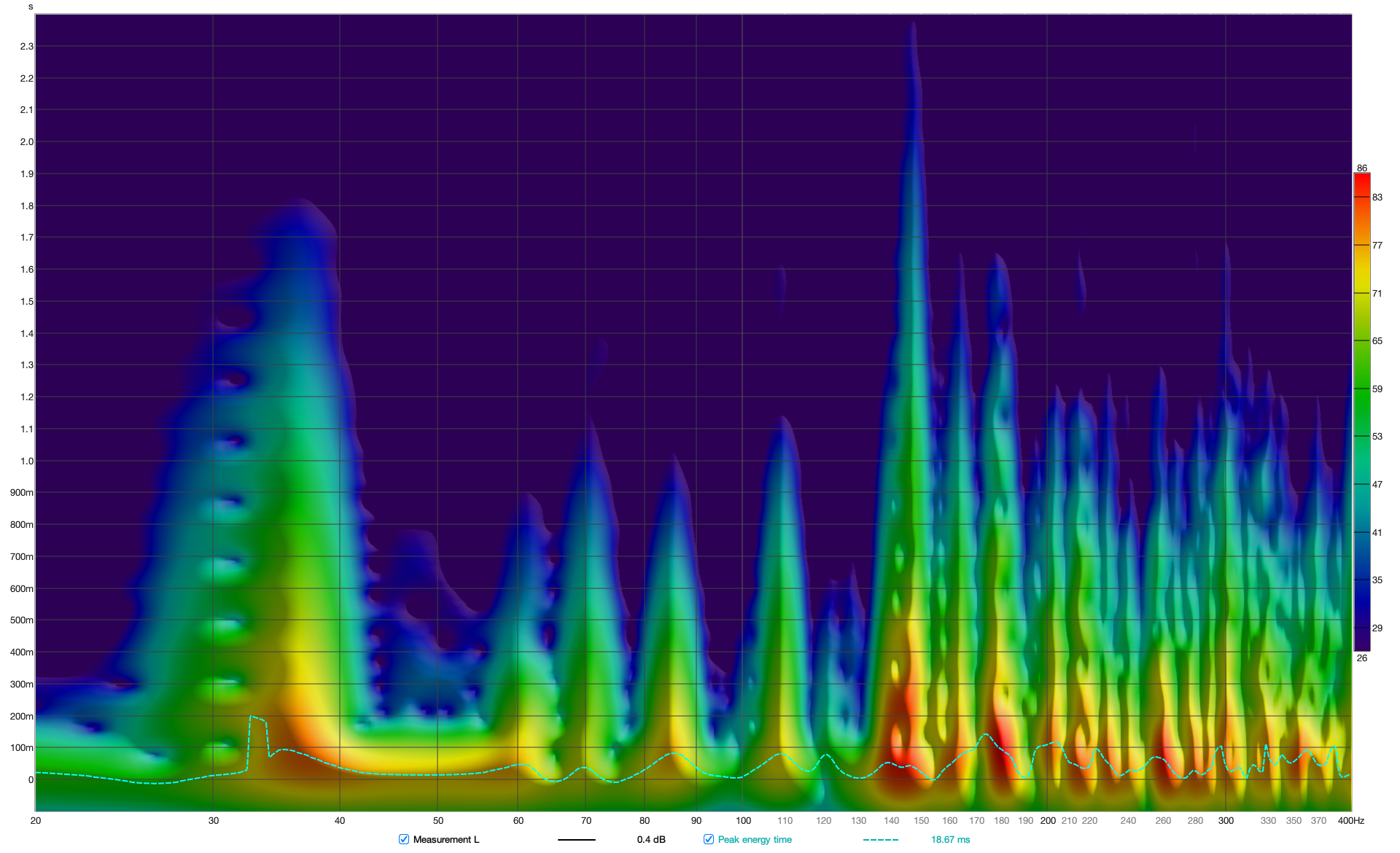
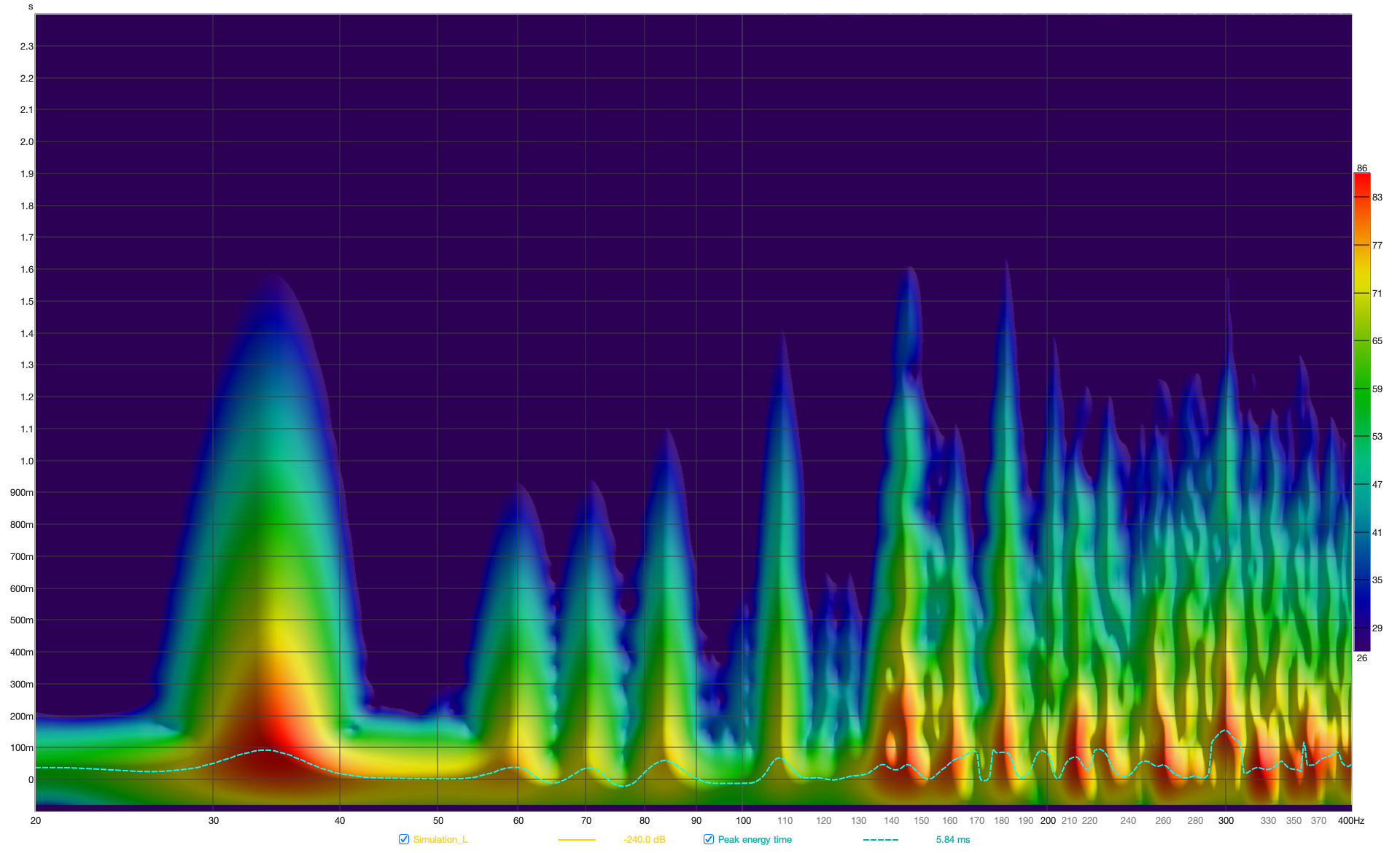
Figure 13 Spectrogram of left loudspeaker from measurement (top) and simulation (bottom)

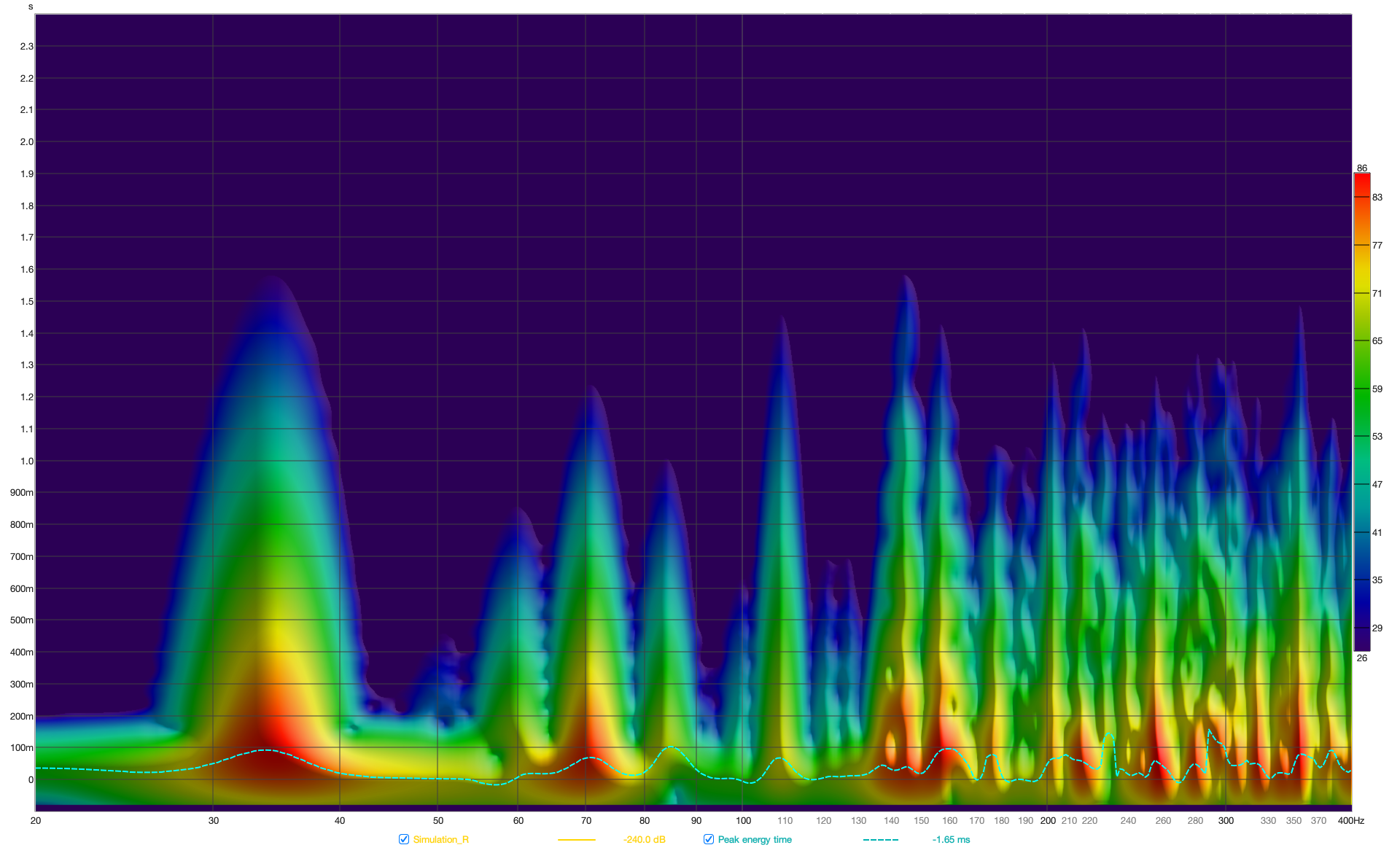
Figure 14 Spectrogram right loudspeaker of measurement (top) and simulation (bottom)

4.3 Single Measurements at the Mix Position

4.4.1 Frequency Response

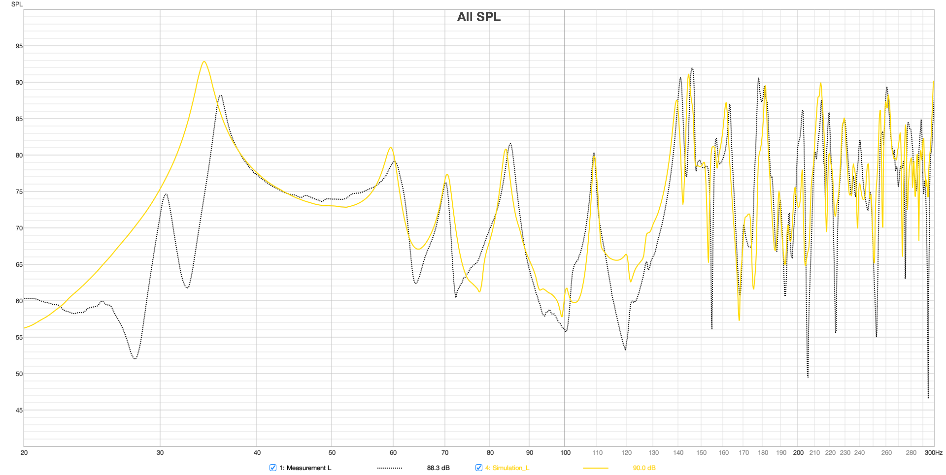
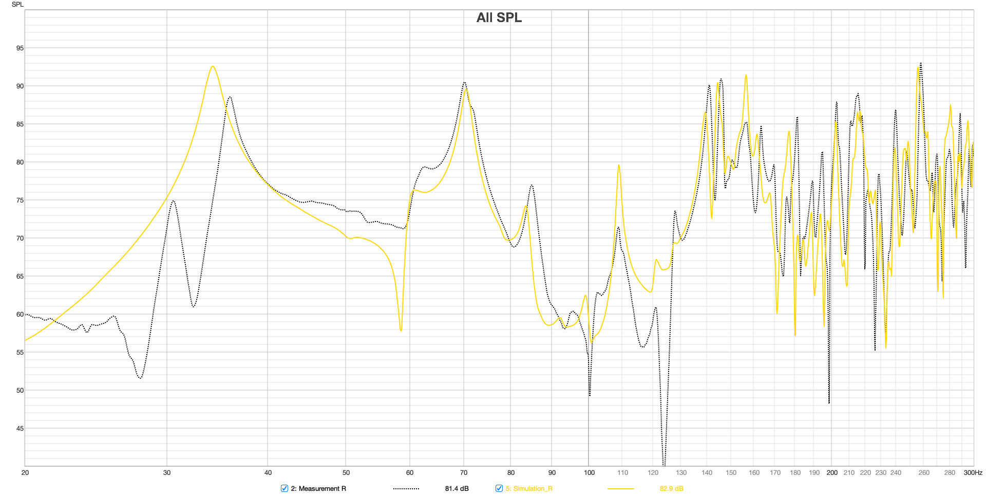
Figure 15 Frequency response measurement and simulation at the listening position 20 - 300 Hz

The frequency responses at the mix position, as shown in Figure 15, indicate a very high level of agreement for both sides. Deviations between simulation and measurement around 58 Hz and in the 100 – 140 Hz range are attributed to the interaction of the speakers with the boundary surfaces and the modeling, as discussed in section 3.3.2 and 3.3.3.

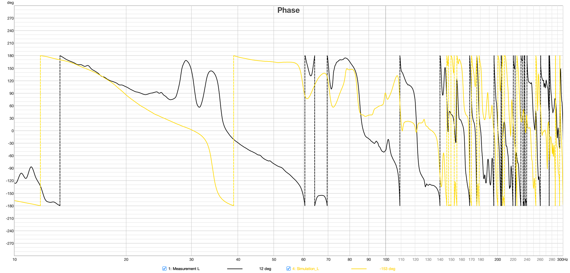
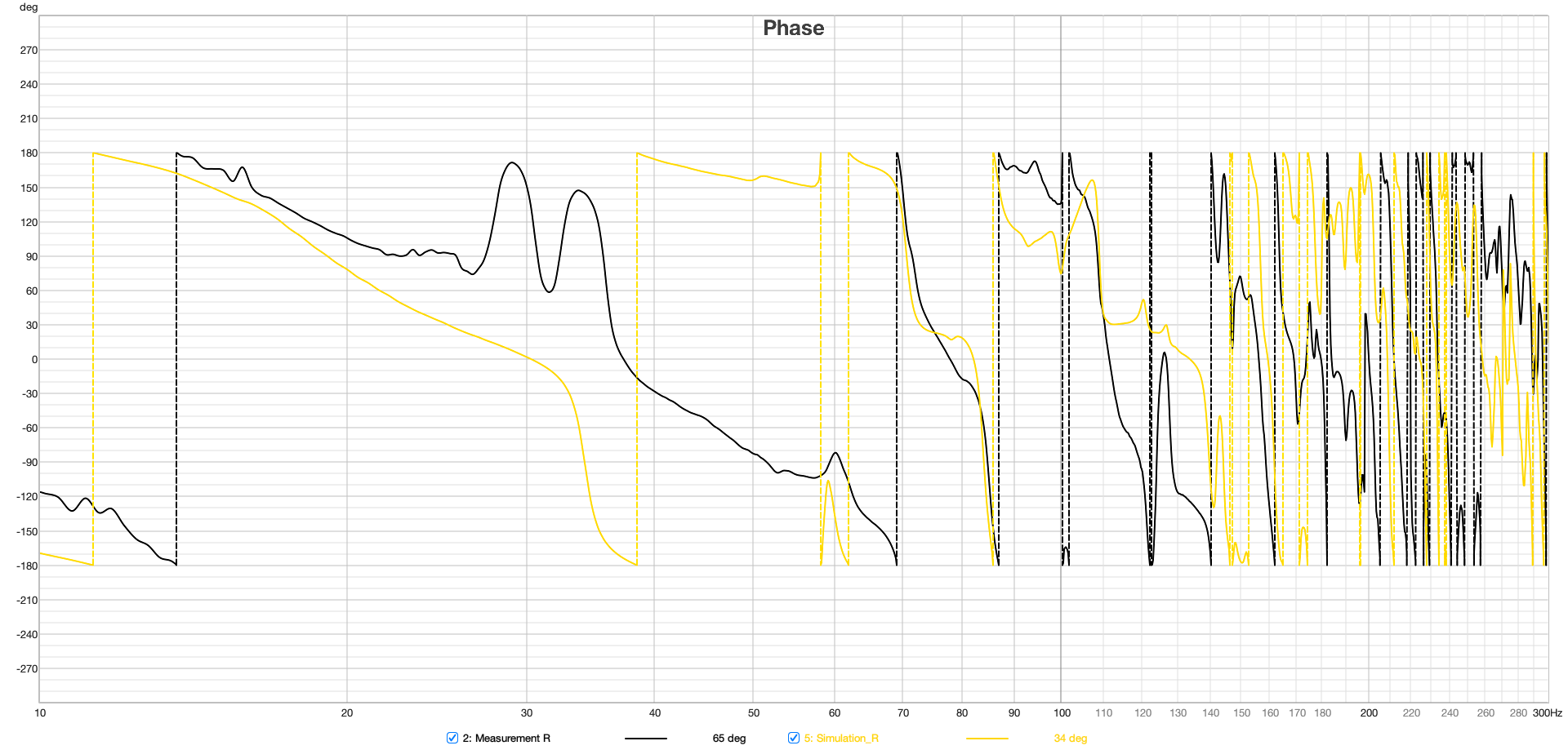
Figure 16 Phase Response Measurement and Simulation at the Listening Position 20 – 300 Hz

The phase responses in Figure 16 of the real and the simulated sound sources show, as expected, significant differences due to the approximation of the sound source, as described in section 3.3.2.

4.3 Sum of Both Speakers

For the validation over the entire measured area, the impulse responses from the simulation of both sources were summed using a Python script and together with the impulses from the measurement, transformed into the frequency domain using an FFT with a resolution of 0.5 Hz. The SPL values were normalized. Subsequently, all data is displayed as a heatmap over the area of the room (see Figure 16). In the simulation, the room modes appear very similar to the measurement. There is a frequency shift of up to 1 Hz in some cases. Slight local shifts between measurement and simulation of the modes on the grid are partly due to inaccuracies in the placement of the measurement positions in the real room, and in some cases, due to the irregular and uneven walls. Mixing position is G7.

4.3.1 SPL Heatmaps

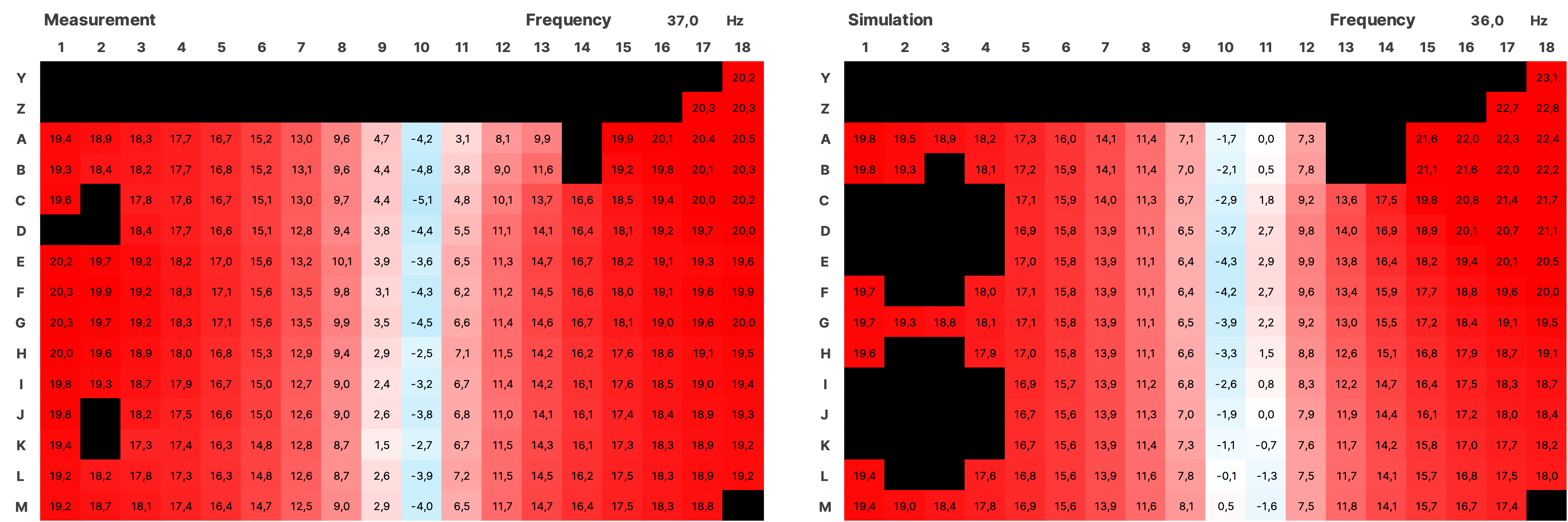
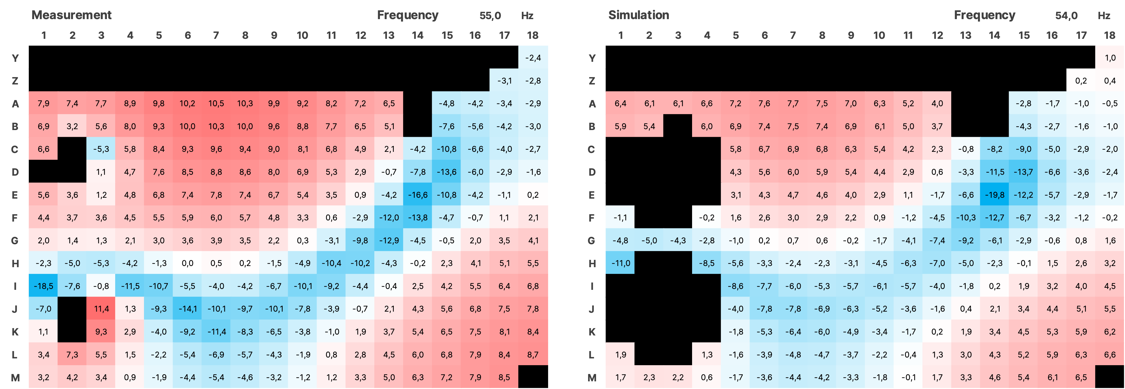
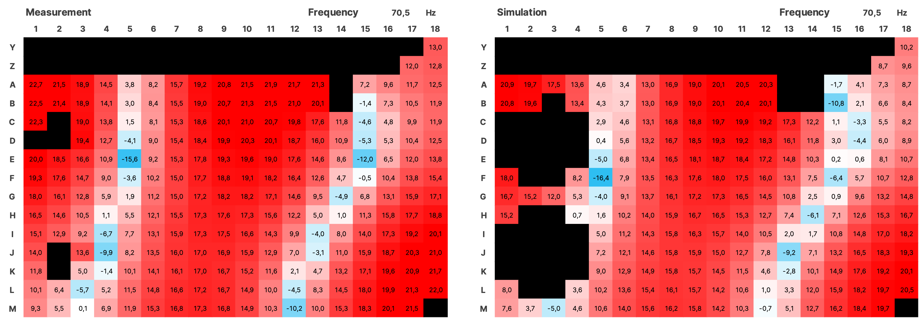
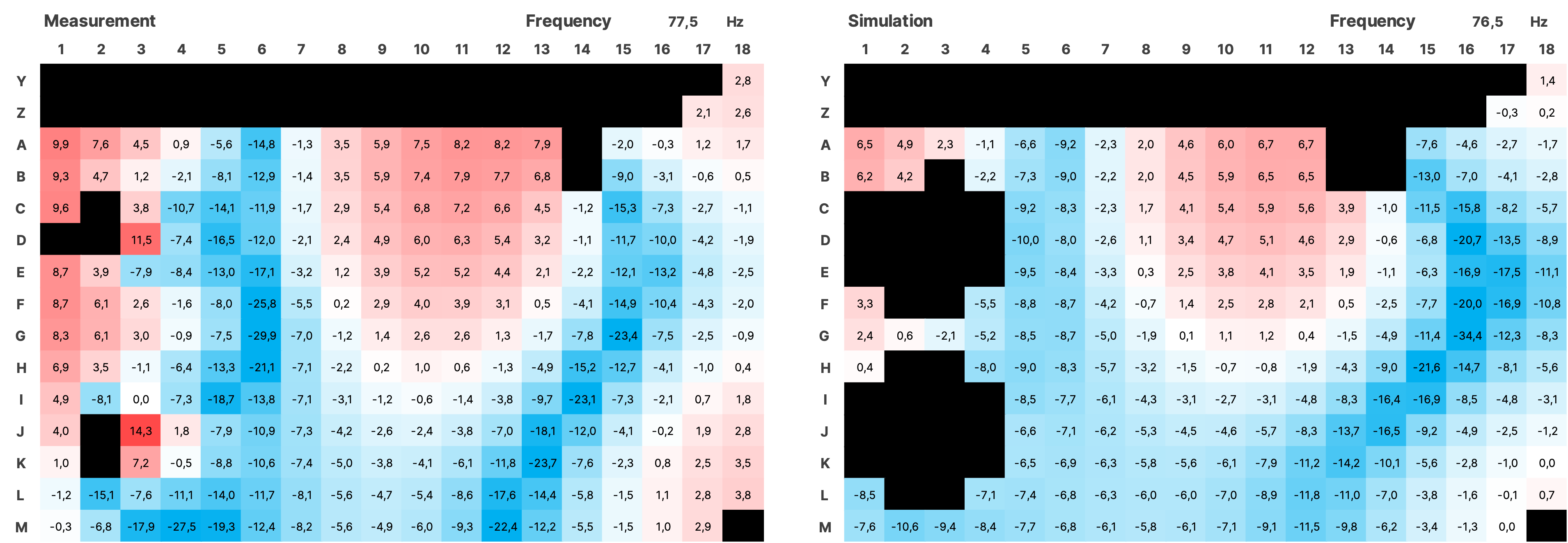
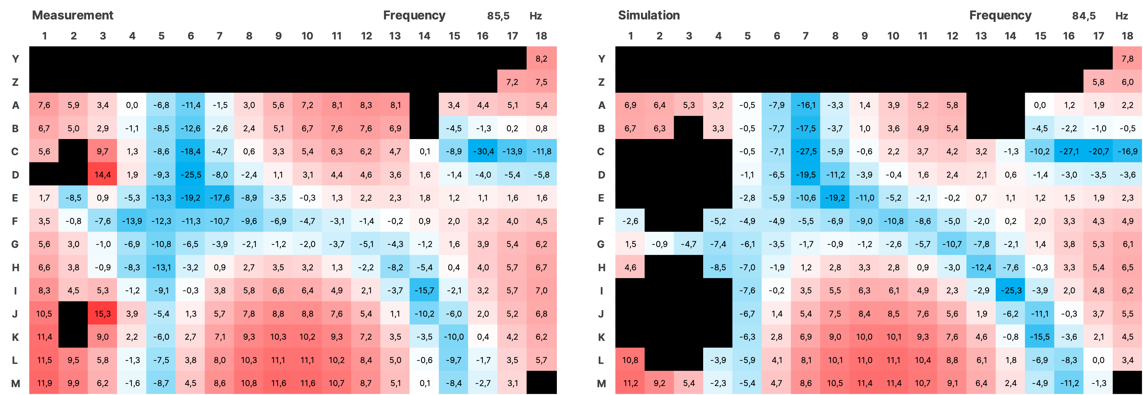
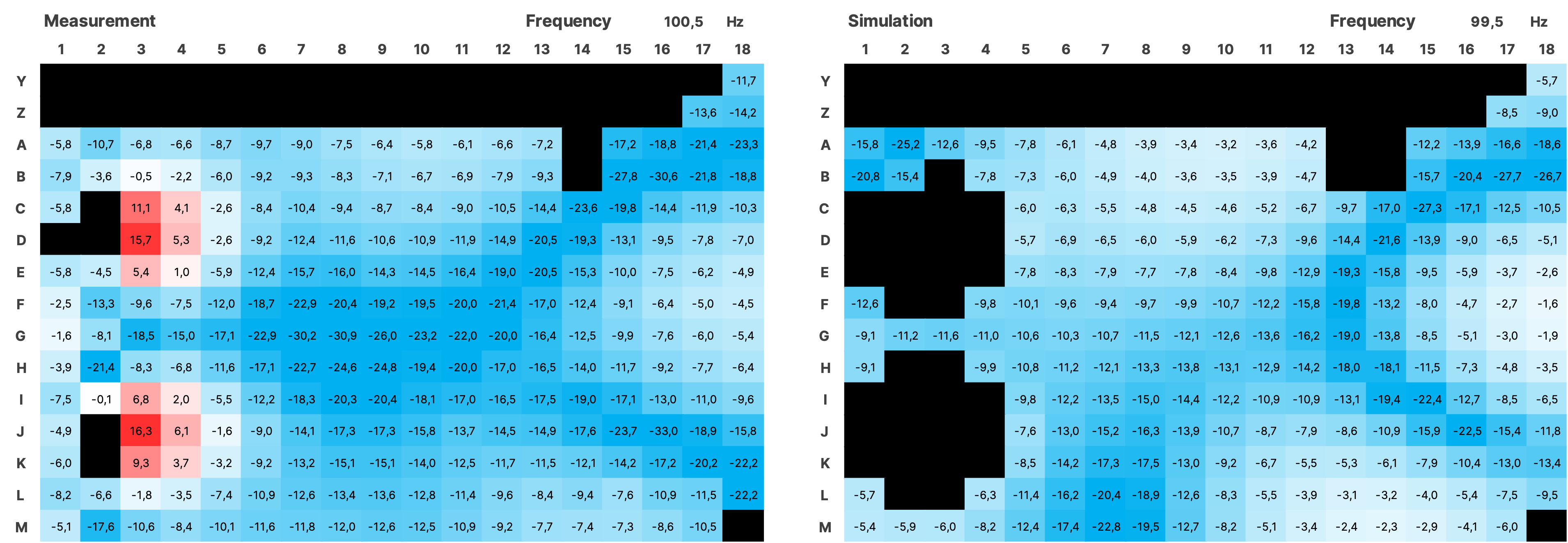
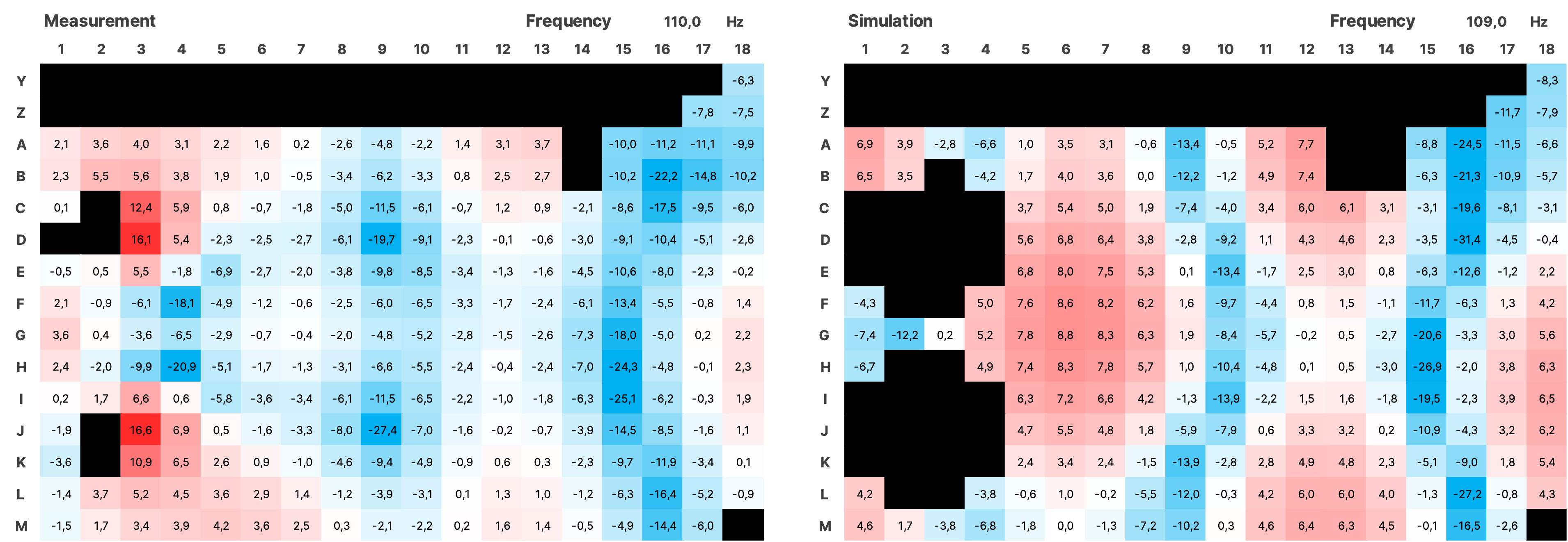
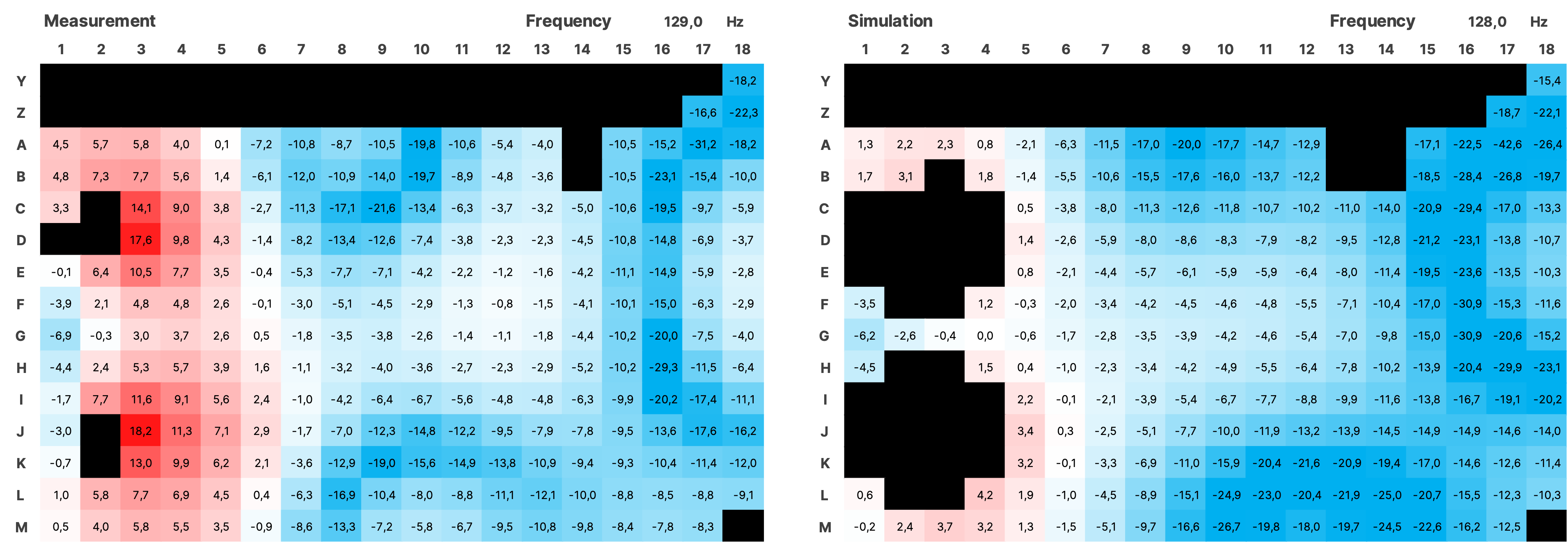
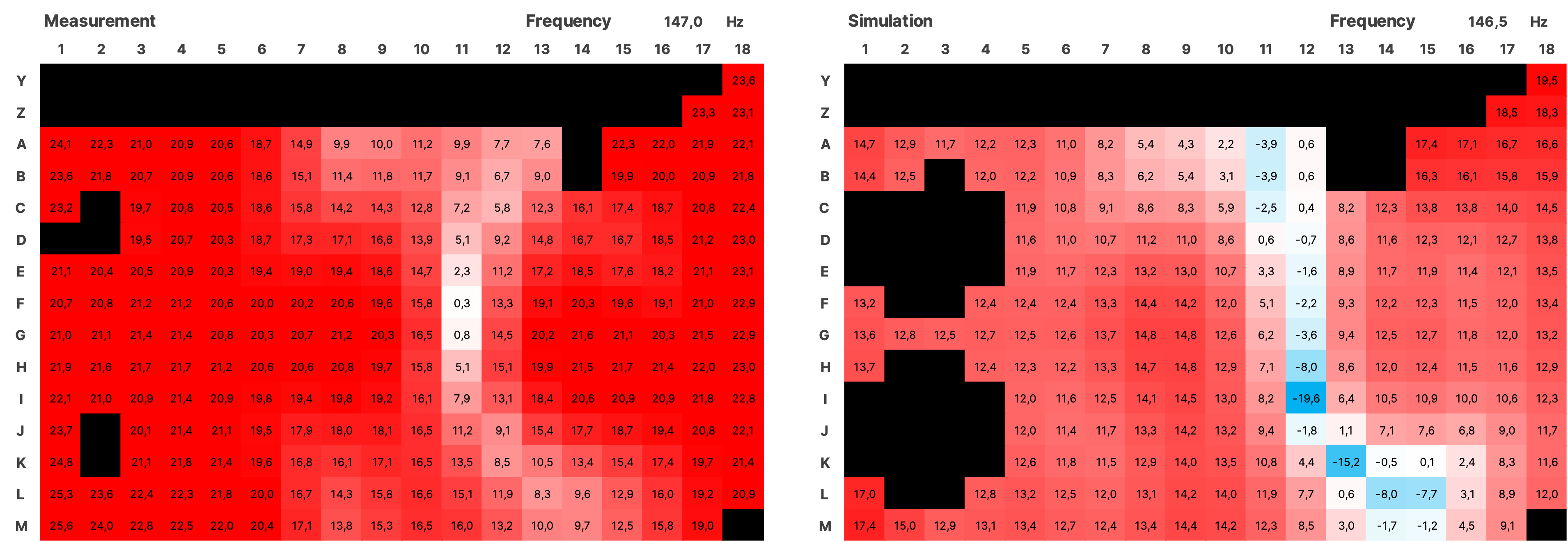
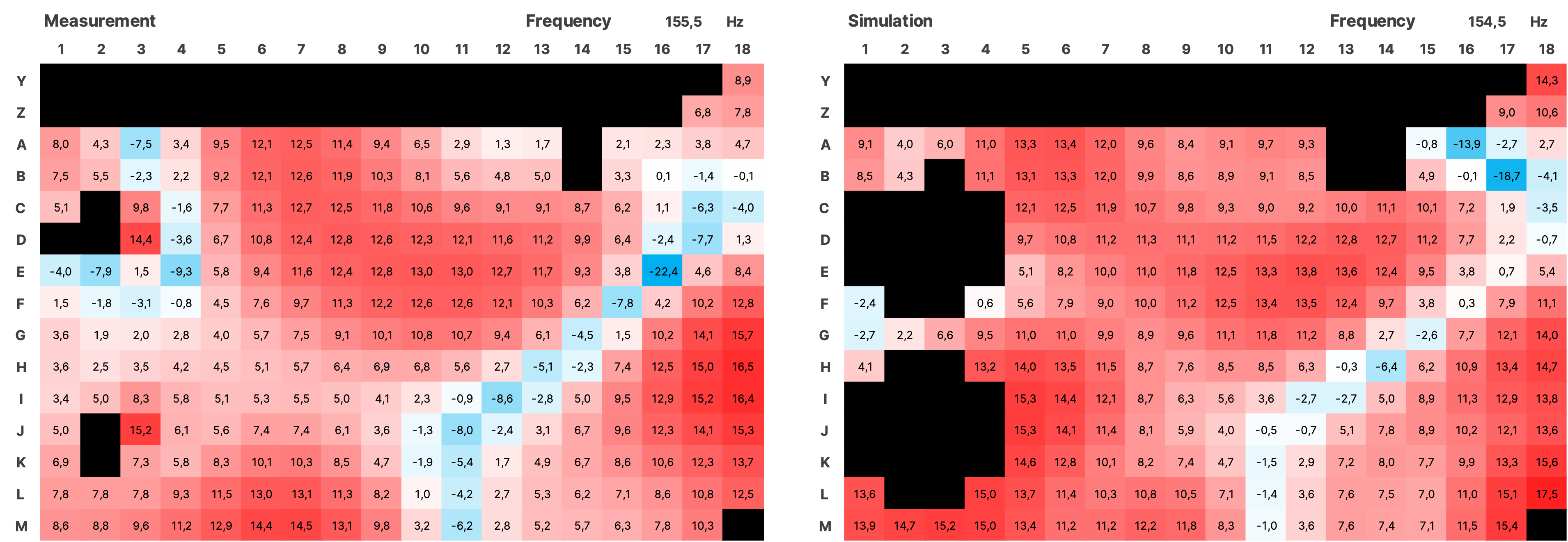
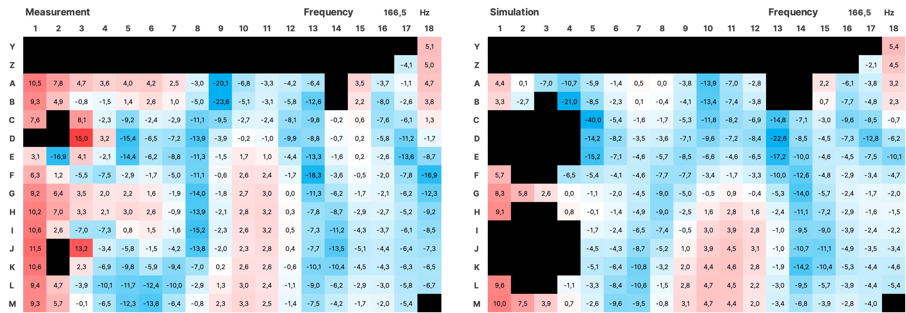
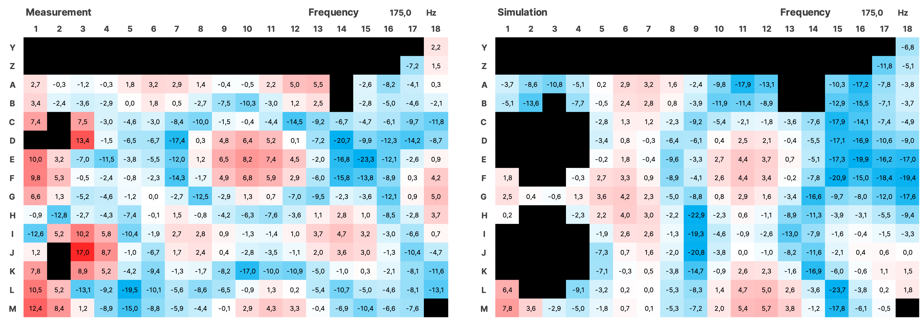
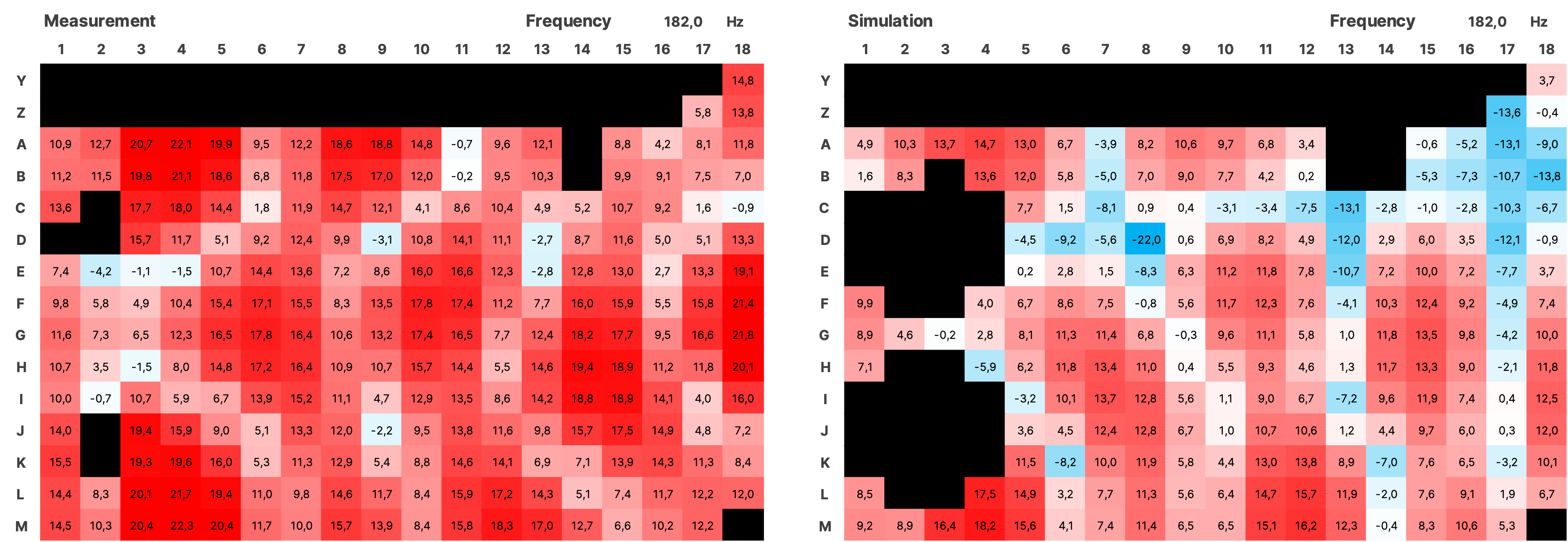
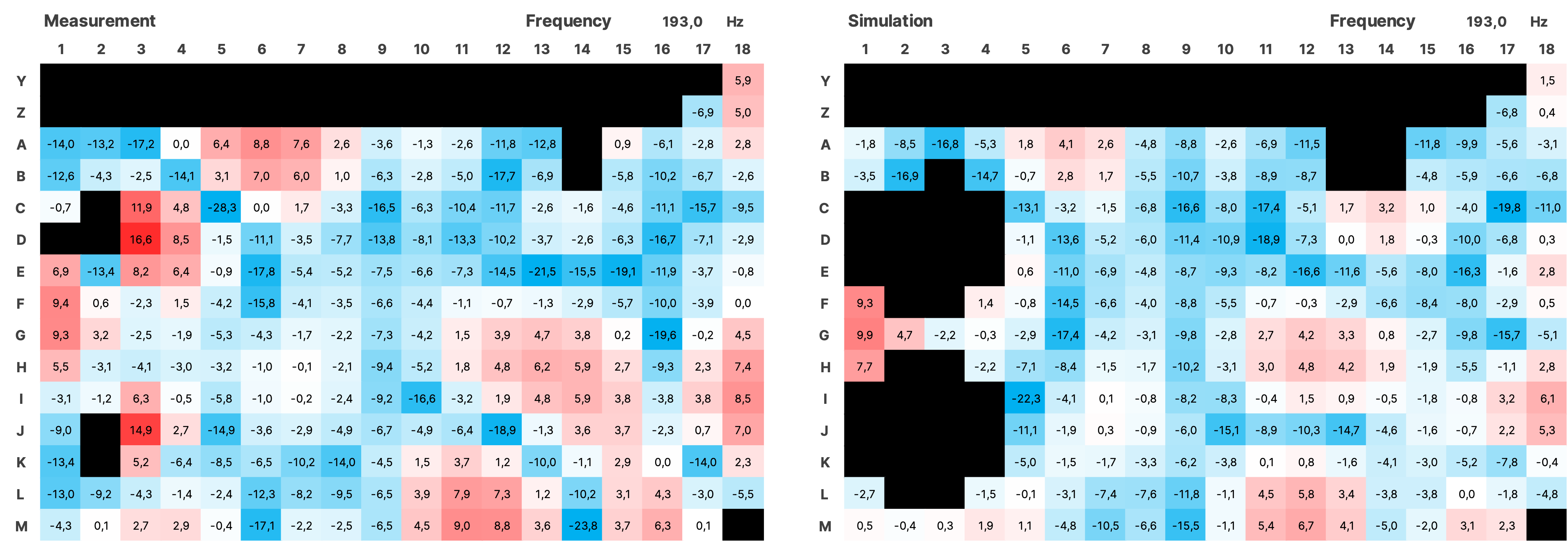
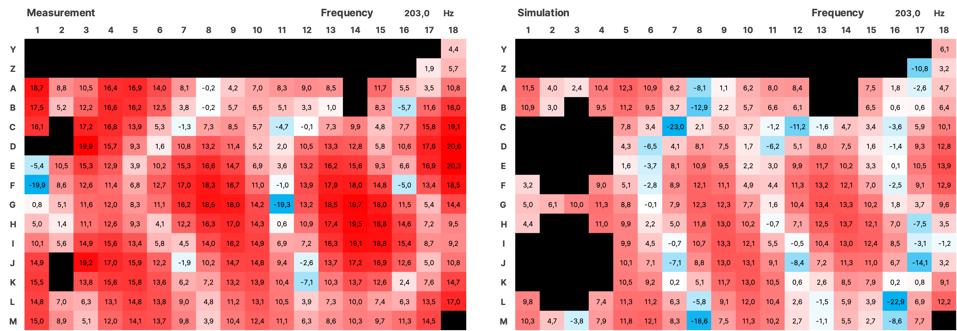
Figure 17 SPL Heatmaps of Selected Frequencies

4.3.2 Frequency Response at Selected Positions in the Room

Despite the large overall agreement between simulation and measurement, the frequency responses of the sum, due to the mentioned differences in the phase responses as seen in Figure 16, show greater discrepancies between the simulation and the actual measurement compared to the individual measurements (Figure 18).

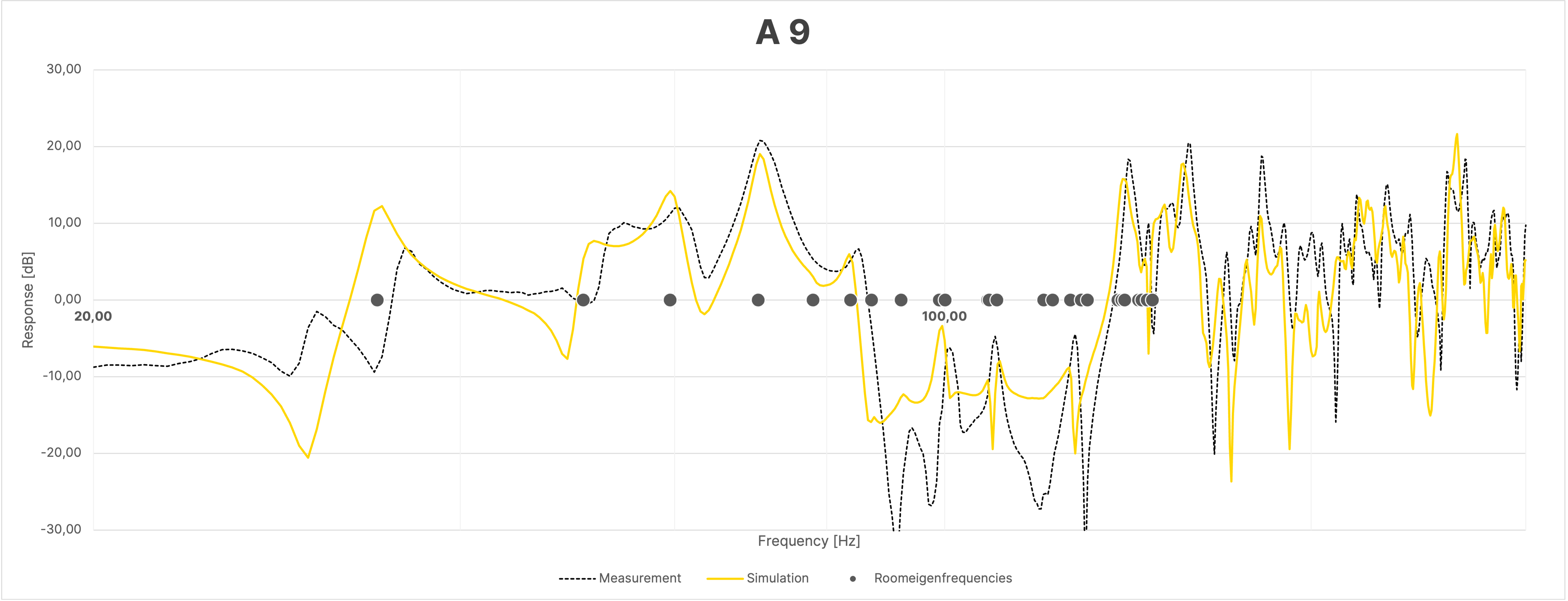
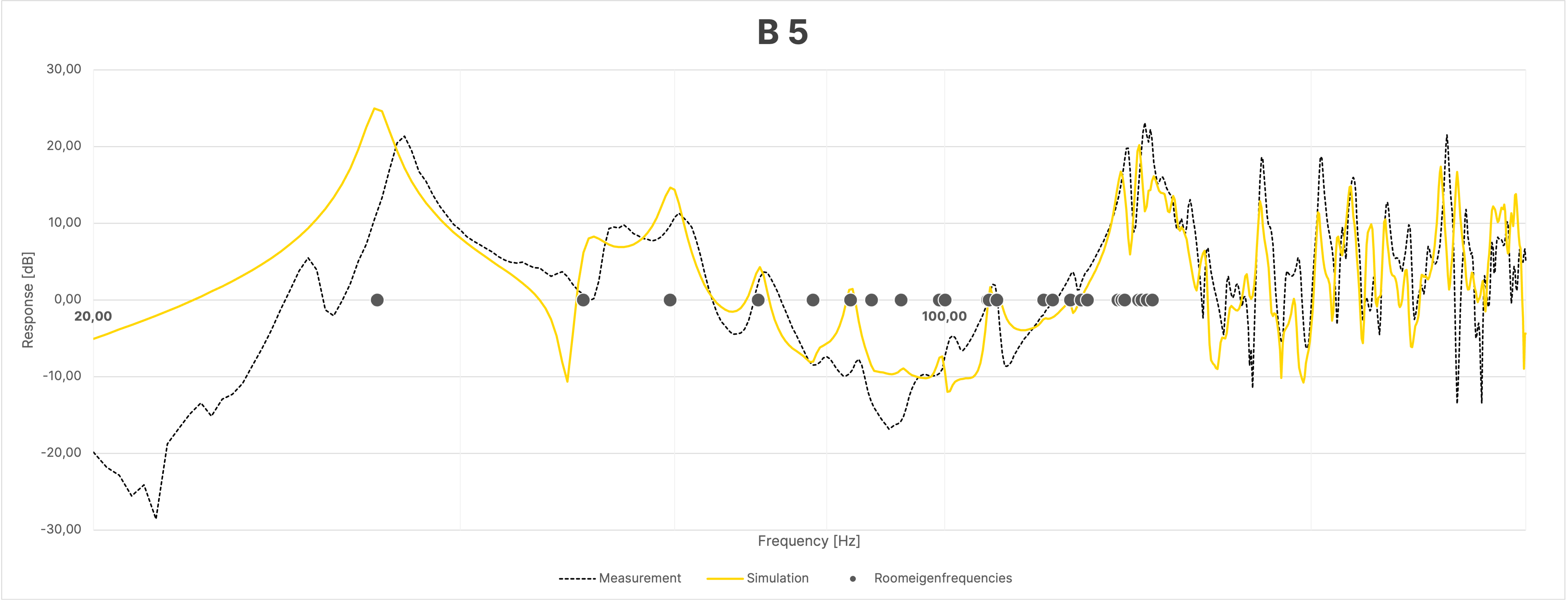
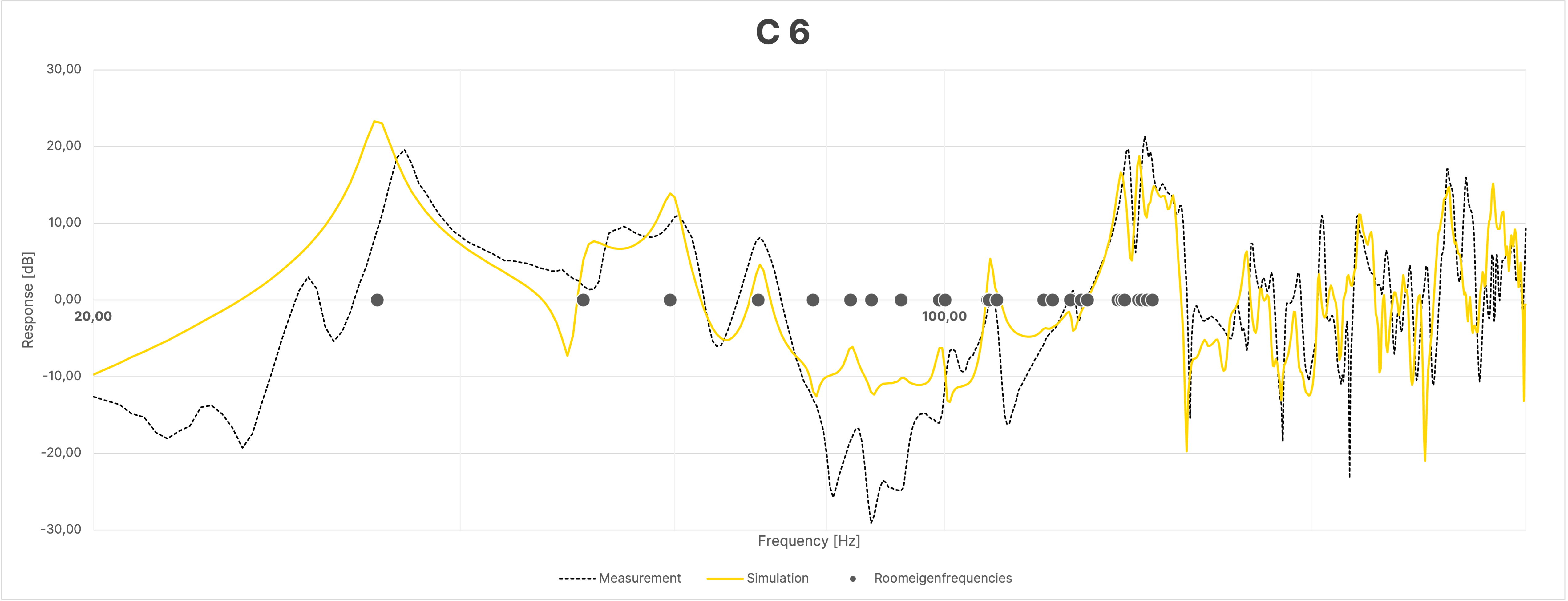
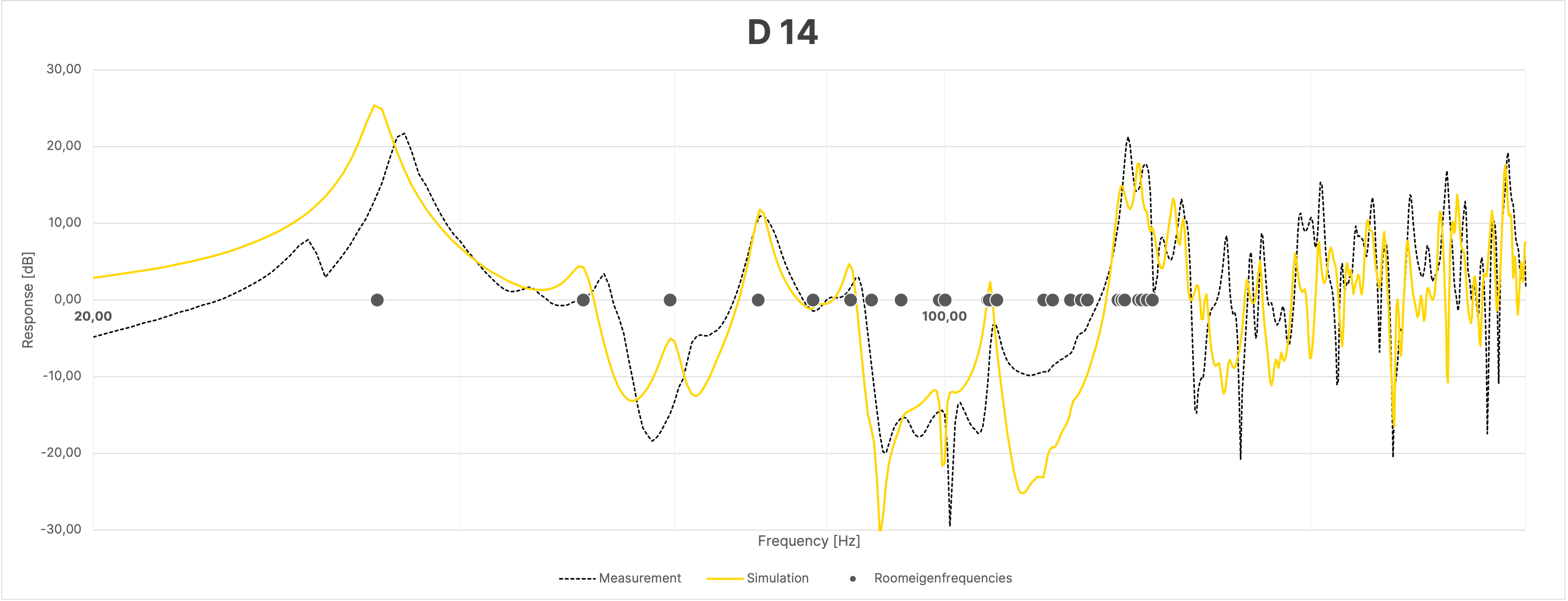
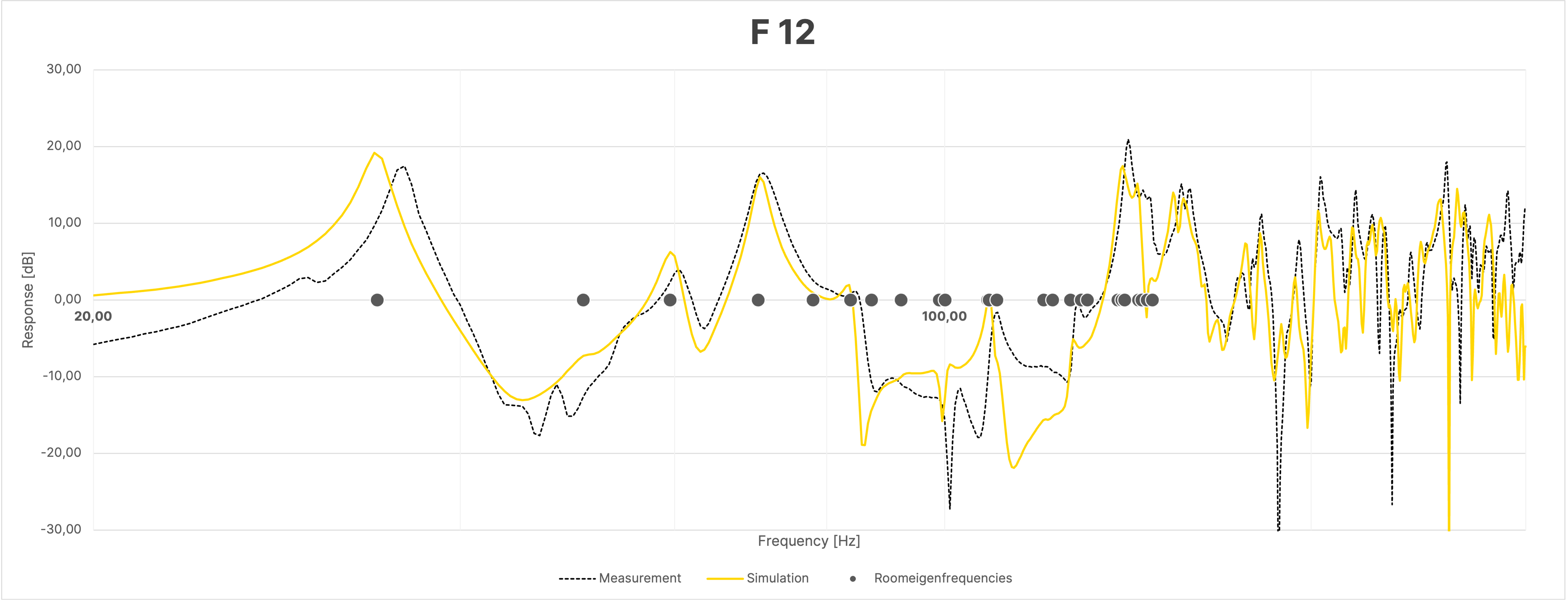
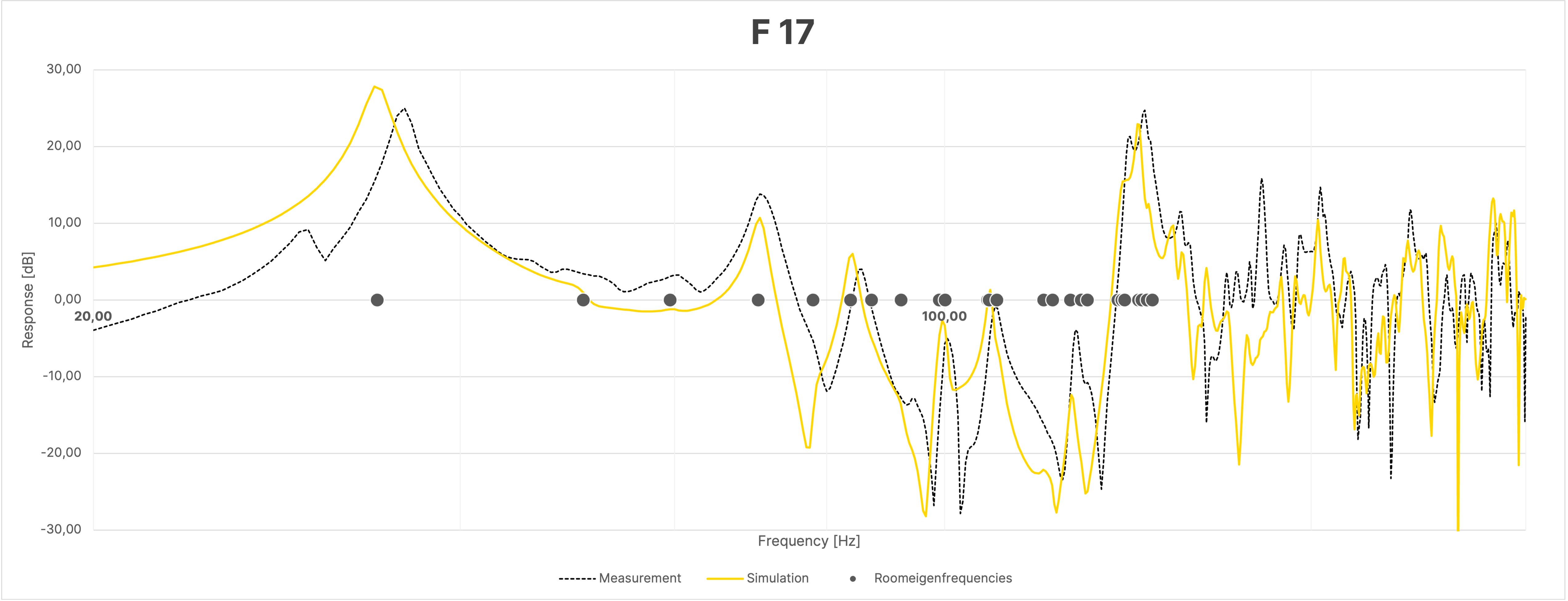
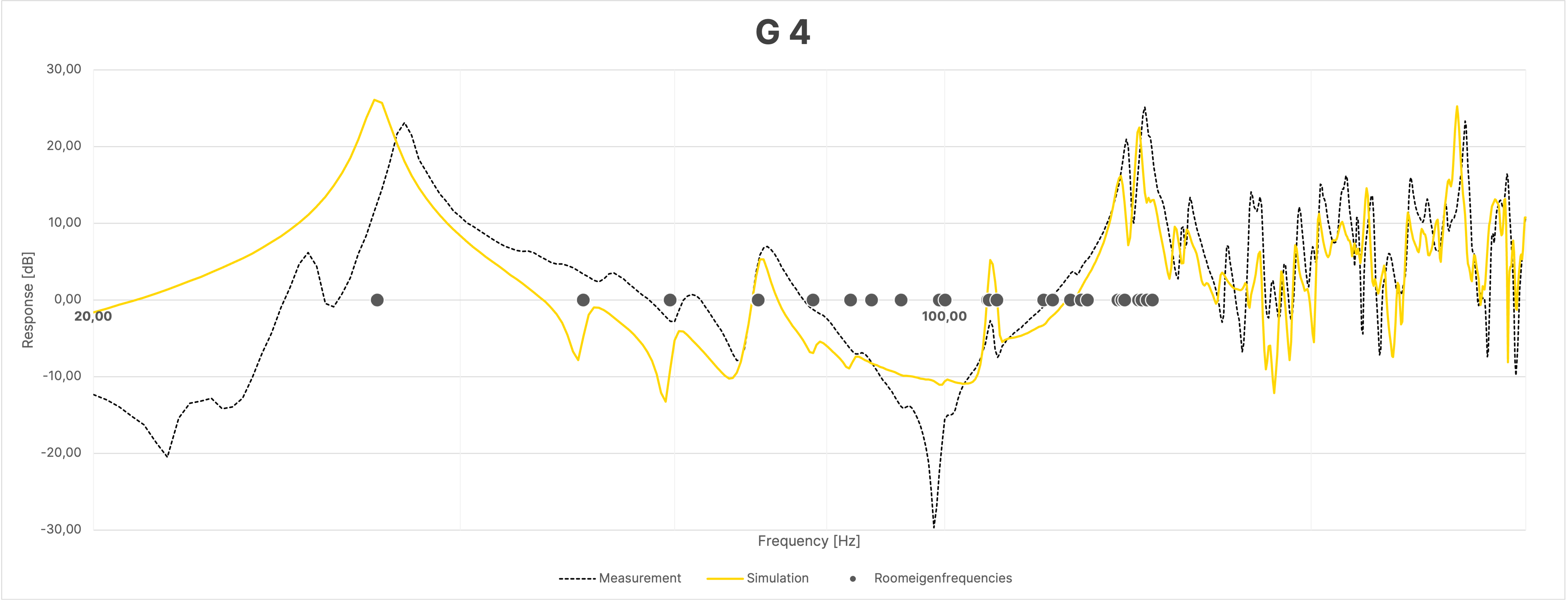
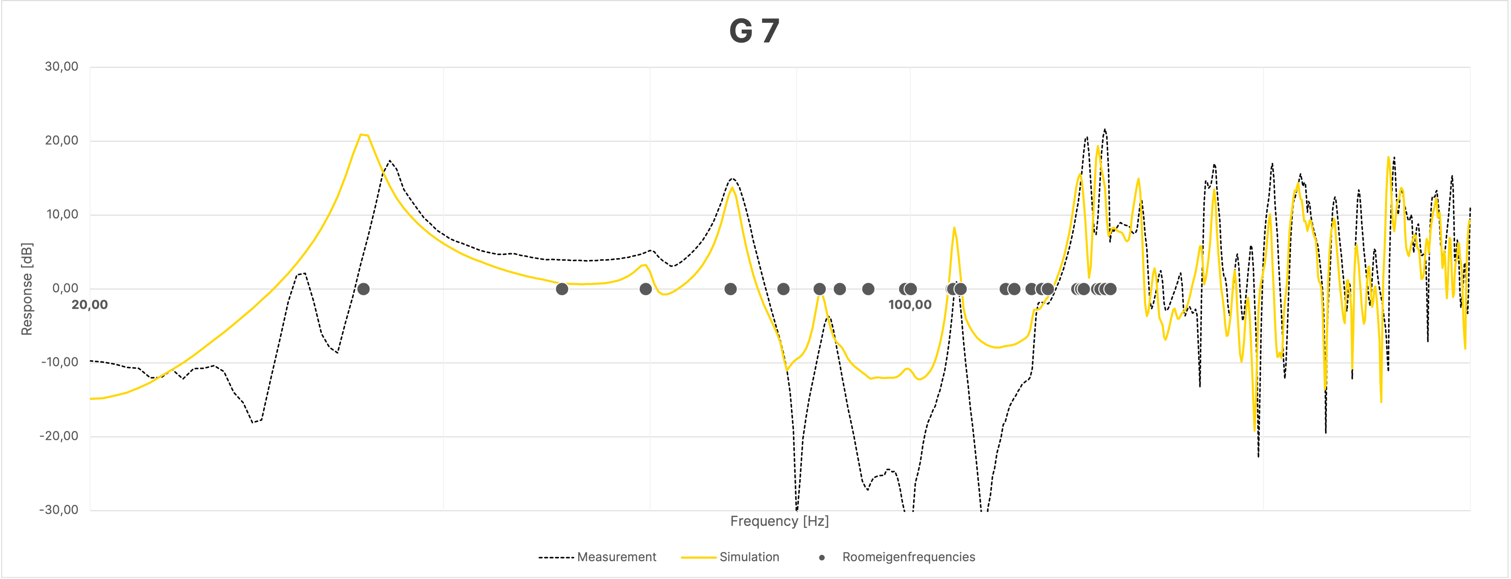
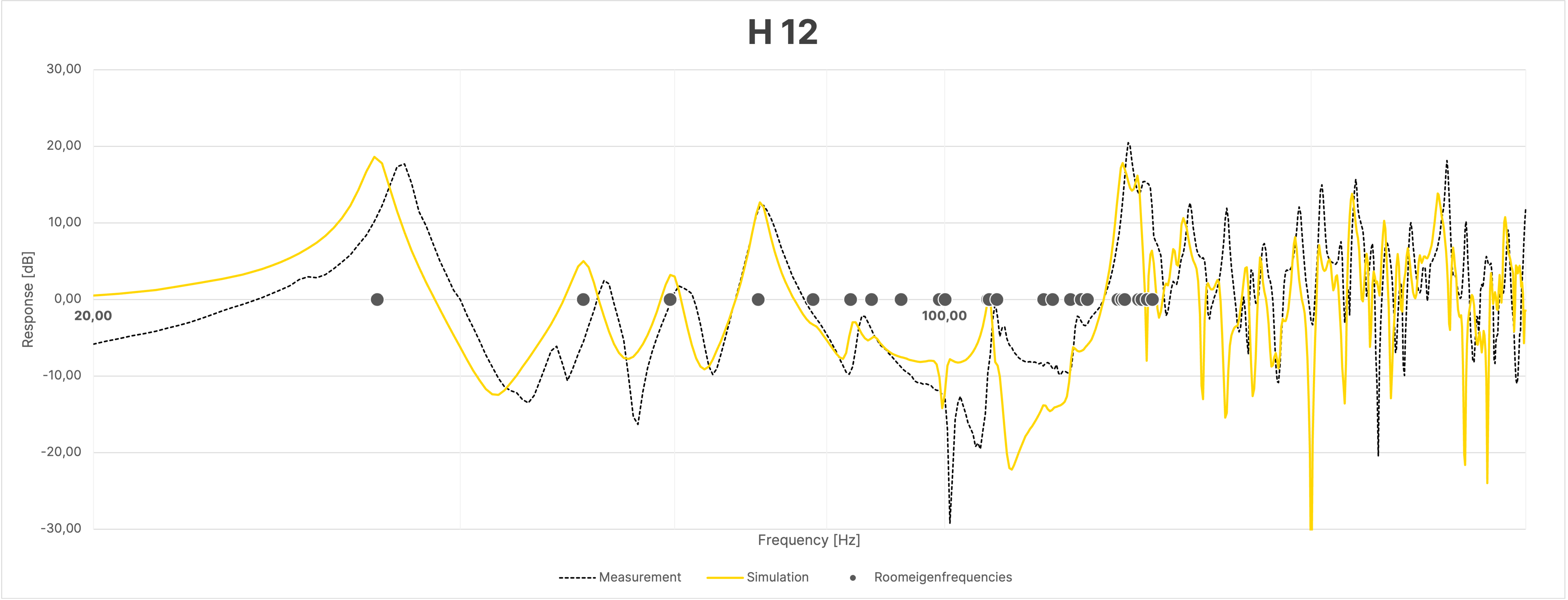
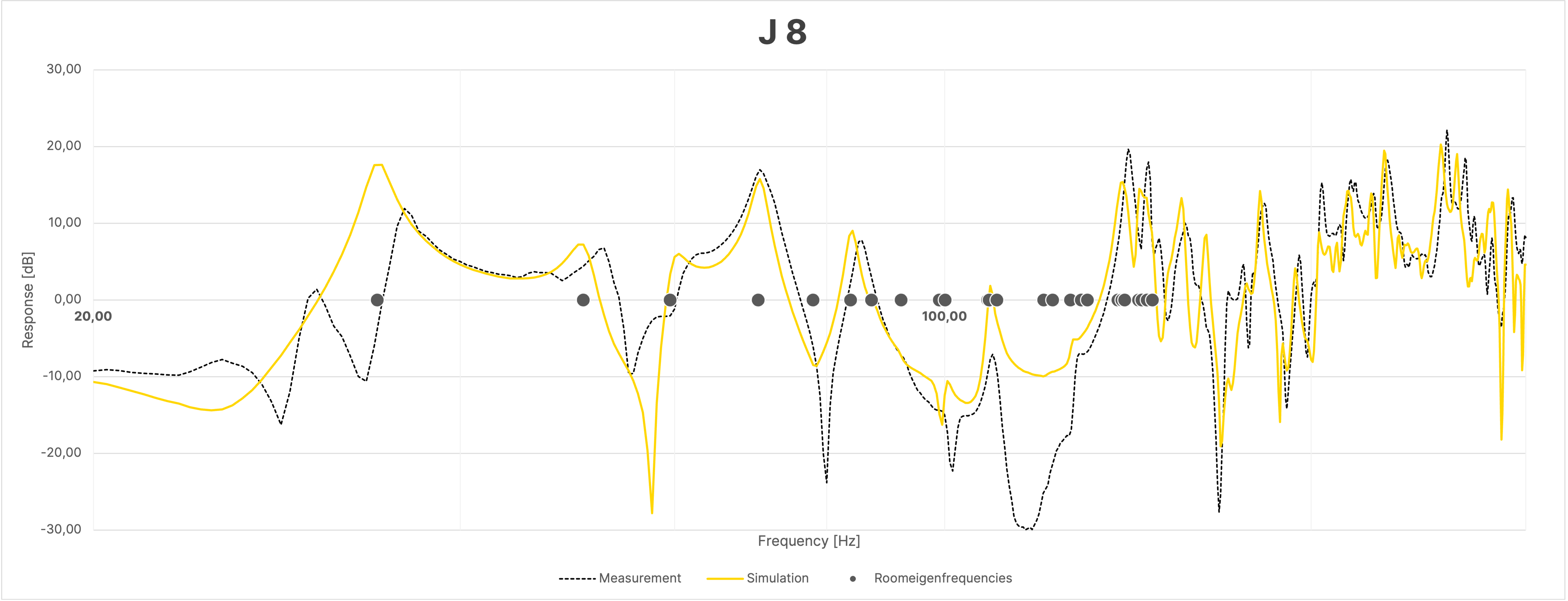
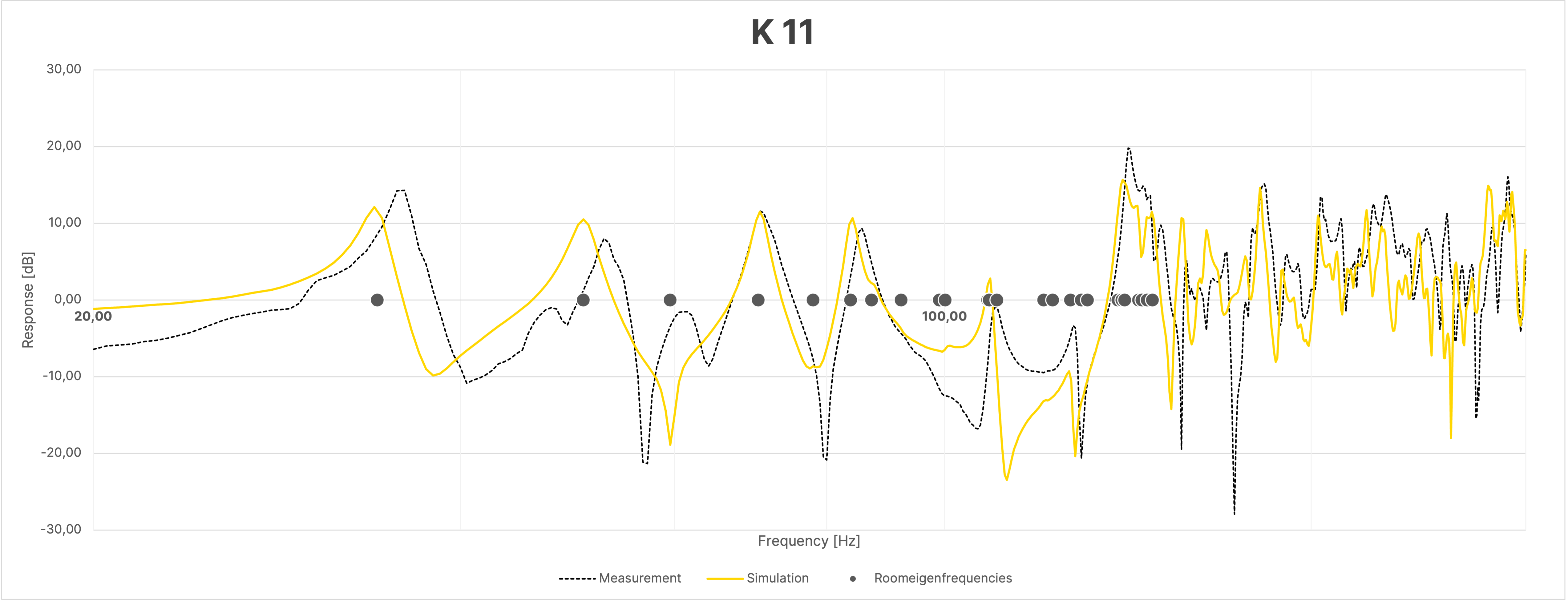
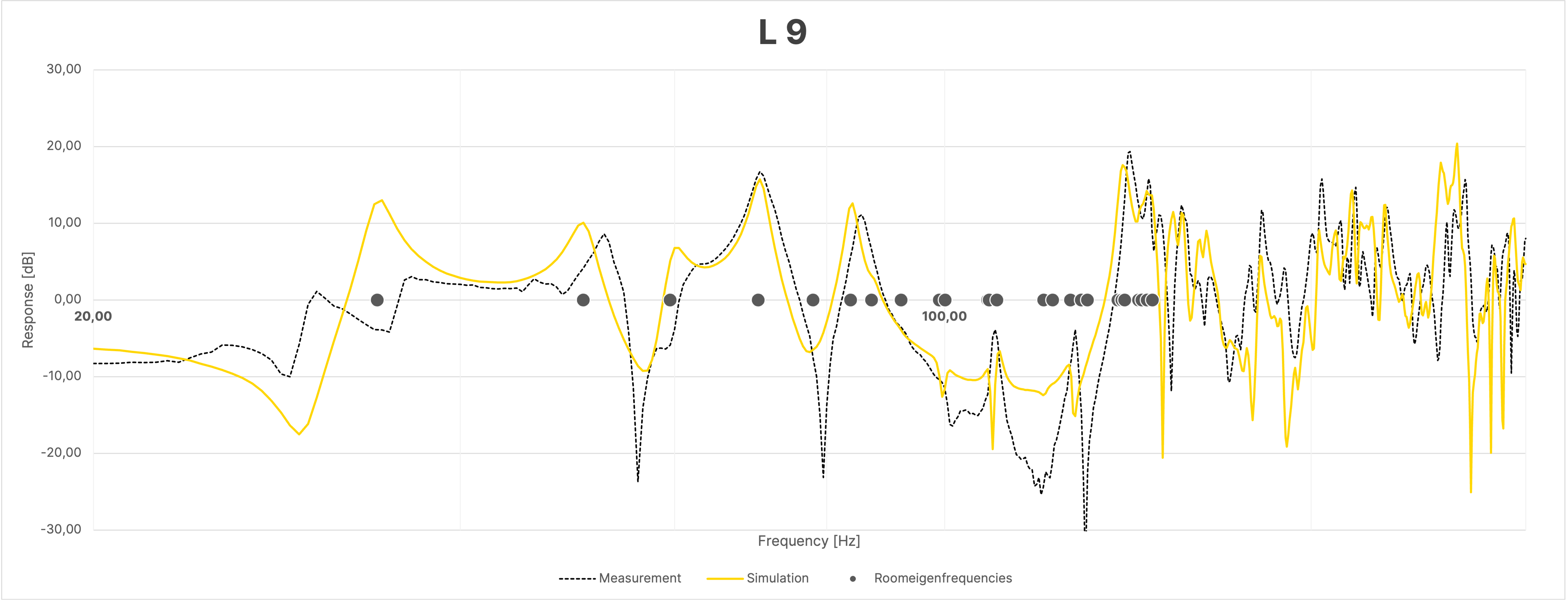
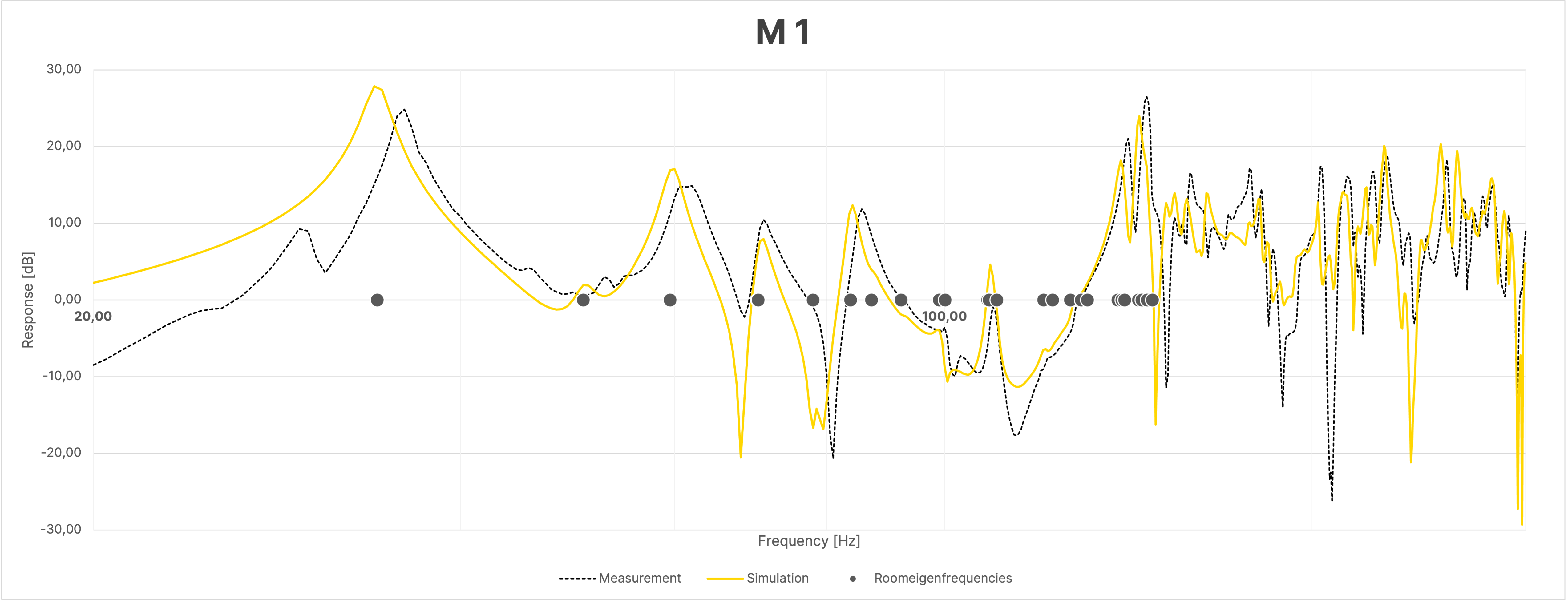
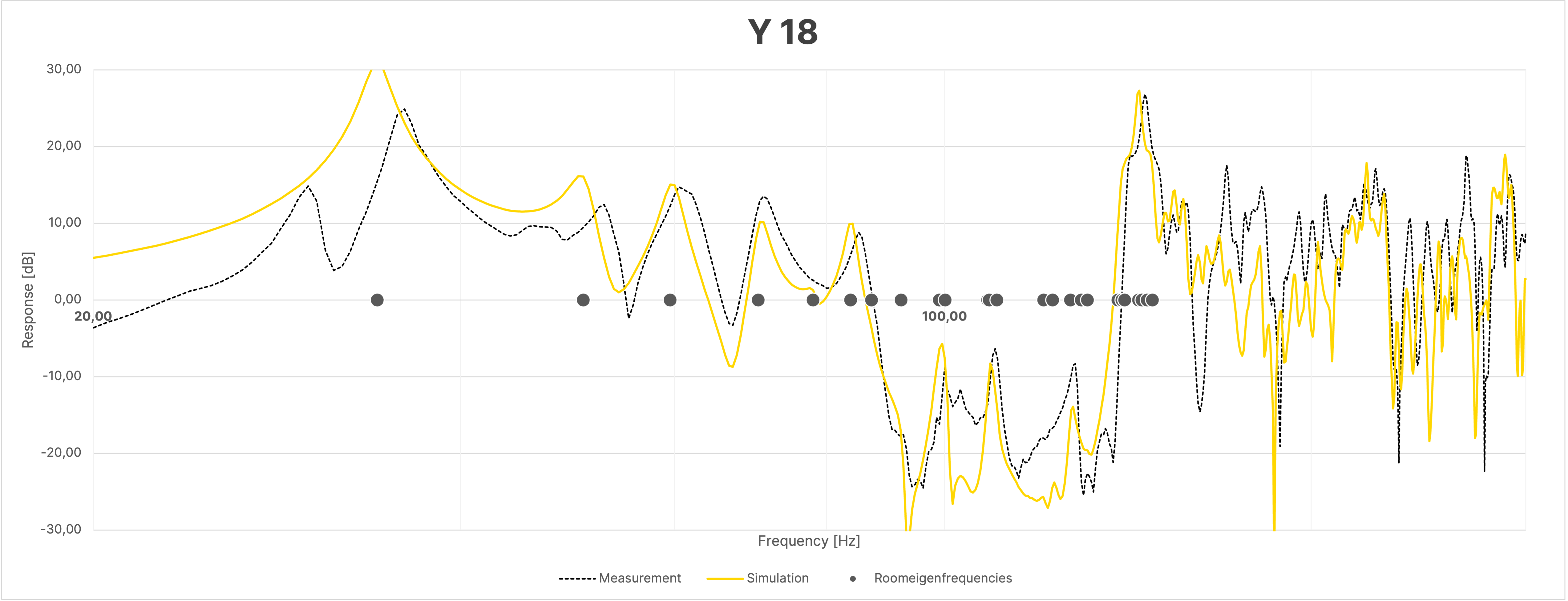
Figure 18 Frequency Response at Selected Positions in the Room

5 Conclusion

Despite the limitations in the modeling of the speakers, the impedances of the surfaces and the uncertainties in the positioning of the measurement points, audics was able to demonstrate that the simulation with the Acoustic Simulation Suite from Treble, particularly the mode field as well as the influence of the boundary surfaces on the speaker reproduction across the entire base area can be captured with high accuracy. Based on the data developed here, optimal positioning of the speakers and planning of acoustic measures are possible, which will be documented in the second part of the case study and eventually validated again through measurements in the final part of the trilogy.

References

AC Acustica. (2023). audieum.com. Retrieved 12. December 2023, from https://audieum.com

Lachot, W. (2016, March). WES LACHOT DESIGN GROUP. Retrieved 12. December 2013, from 10

TIPS FOR SMALL- ROOM ACOUSTICS: http://weslachot.com/articles.html#image23

LoudspeakerTechnologyLtd. (2023). atc.audio. Retrieved 12. December 2023, from TECHNICAL DATA SHEET SCM25A Pro Mk2: http://atc.audio/wpcontent/ uploads/2023/07/ATC_SCM25A_Pro_Mk2_TDS_revB.pdf

Mellor, N. (2016, March). ACOUSTIC FRONTIERS. Retrieved 12. December 2023, from WELCOME TO ACOUSTIC FRONTIERS BLOG: https://acousticfrontiers.com/blogs/acousticanalysis/ what-is-speaker-boundary-interference

Mulcahy, J. (2022). roomeqwizard.com. Retrieved 12. December 2023, from RT60 Decay Graph: https://www.roomeqwizard.com/help/help_en-GB/html/graph_rt60decay.html

Post Scriptum Audio. (2023). postscriptumaudio.com. Retrieved 12. December 2023, from https://www.postscriptumaudio.com

Treble Technologies. (2023). treble.tech. Retrieved 12. December 2023, from Converting absorption coefficients to reflection coefficients: https://docs.treble.tech/materialinput/

Tripp, K. (2022). Ken's Audio Page. Retrieved 12. december 2023, from SBIR and floor bounce calculator: http://tripp.com.au/sbir.htm