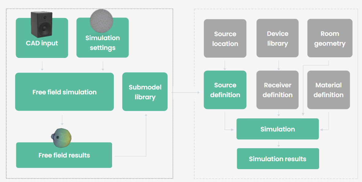
Boundary Velocity Submodels
A boundary velocity source is an advanced sourcetype in the treble engine that uses a the boundary velocity layer source on an injected geometry of the source for the dg solver and a directional points source in the ga solver, thereby also enabling hybrid simulations with this source type. This enables a highly accurate source characterstics in the low frequencies with near field effects, along with a highly flexible model in the high frequencies by using a directional point source. The source submodels can be created directly in the SDK using the free field simulations.
Creation
A boundary velocity submodel can be created from a free field simulation.
#fetch the simulation from the project
ff_simulation = project.get_simulation_by_name('my_ff_model')
# Get the results object
ff_results_obj = ff_simulation.get_results_object(f"/tmp/{ff_simulation.id}")
ff_submodel2k = ff_results_obj.create_boundary_velocity_submodel(submodel_name, "")
Usage
The boundary velocity submodel source is used like a directional point source:
my_submodel = tsdk.boundary_velocity_submodel_library.get_by_name("MySubmodel")
source = treble.Source.make_boundary_velocity_submodel(
    position=treble.Point3d(5,2,1.2),
    orientation=treble.Rotation(azimuth=42),
    boundary_velocity_submodel=my_submodel,
    label="MySubmodelSource"
)
This source can then be used as an input to a simulation in the SimulationDefinition, where the source list can contain multiple different source types.
Boundary velocity submodel concept
The boundary velocity submodels are essentially an automation of the boundary velocity layer source. When a submodel source is used in a dg or hybrid simulation the mesh used in the dg solver will be have actual geometry of the source injected into the mesh. This is the geometry that was used to create the submodel source in the first place using the free field simulation. The dg part of the simulation will the automatically assign the right boundary and mesh configuration for the source geometry so the model is excited in exactly the same way as it was in the free field simulation. A postprocessing step will the use a custom source correction filter that also was extracted in the free field simulation. This source correction filter will ensure that the on-axis response is a flat 1Pa at 1m distance from the source in anechoic condition. This enables the source to be placed anywhere in the model as long as the radiating membrane of the model is not intersected by the geometry of the model.
The interaction between the near-field of the speaker and the model geometry is expected to have an influence on the sound field, e.g. the effect of placing a loudspeaker in the corner of the room. This is indeed also the expected outcome of the simulation to include these effects, but it will also have the influence that the speakers radiation pattern is no longer flat in the frequency domain. There reference for the flat frequency response is always the anechoic condition as is the expection in real life measurements as well where the environment most often has a profound effect on a sound source's ability to radiate sound.
The when running a ga or a hybrid simulation, the ga solver always receives the pattern that was extracted from the free field simulation. i.e. the far field approximation of the response in 5 deg azimuth and elevation steps. This functions exactly as the normal directive point source, which does not inherently model near field effects, so use caution for the high frequency response when evaluating the repsonse very close to the source.
It is currently not possible to input an on-axis response to the boundary velocity submodel sources, however the on axis response can be customized at a later stage using the .filter() functionality on the IR objects using the results object.
Boundary velocity submodel library
The boundary velocity sumbodels can be accessed and managed from the boundary velocity submodel library tsdk.boundary_velocity_submodel_library. It is for example possible to use .delete() or .rename_submodel to manage the organizational wide database of models. Use the .plot_directivity_pattern() on a fetched source to visualize the directivity pattern.