Loudspeaker Modeling using Boundary-velocity Submodels
Introduction and background
This article validates the boundary-velocity submodel feature of the Treble SDK using two loudspeaker case studies. In each case, we compare simulated and measured acoustic responses under anechoic conditions at multiple angles around the loudspeaker, at a radial distance of 1 meter.
The first case study is a single-driver loudspeaker (Avantone MixCube), simulated using the wave acoustics (DG) solver up to 11,000 Hz. The simulated directivity agrees well with measurements across the full bandwidth.
The second is a two-way studio monitor (Yamaha H8), which uses separate drivers for low and high frequencies (woofer and tweeter). This example extends the validation to a multi-driver configuration and directly compares two simulation strategies: a fully wave-based simulation using the DG solver against a hybrid simulation in which the tweeter is modeled using the geometrical acoustics (GA) solver. Both strategies reproduce the measured directxivity well, and their results are nearly identical across the full frequency range.
Boundary-velocity submodels
Boundary velocity submodels are a Treble SDK feature for embedding a loudspeaker's geometry directly into a room simulation, based on pre-computed free-field simulations of the source. The loudspeaker's influence on the surrounding sound field, including scattering and diffraction around the enclosure, is therefore captured automatically.
Each submodel includes a correction filter that normalizes the source to a flat 1 Pa on-axis response at 1 m under anechoic conditions, providing a consistent reference level independent of the loudspeaker's own frequency coloration.
When using the DG solver, the submodel automatically applies boundary conditions and mesh refinement at the source geometry, enabling accurate modeling of diffraction and other wave effects. In a hybrid simulation, the GA solver instead represents the source as a directive point source whose directivity pattern is derived from the free-field results.
Experimental setup
Both case studies share the same source-receiver configuration and experimental procedure. The loudspeaker is placed at the center of a room, with a semicircular array of 19 microphone positions arranged at 10° intervals along a 1-meter radius arc. The array spans 0° to 180° counter-clockwise, with 0° defined as the loudspeaker's on-axis (forward-facing) direction, as illustrated in Figure 1.
Measurement
We conducted measurements in a semi-anechoic chamber. We captured acoustic impulse responses at each receiver location using a swept sine method: a 10-second logarithmic sine sweep from 50 Hz to 20 kHz. A GRAS 1/2'' free-field microphone was used with 24-bit/48 kHz sampling. We located receiver positions using a 1-meter string and a protractor.
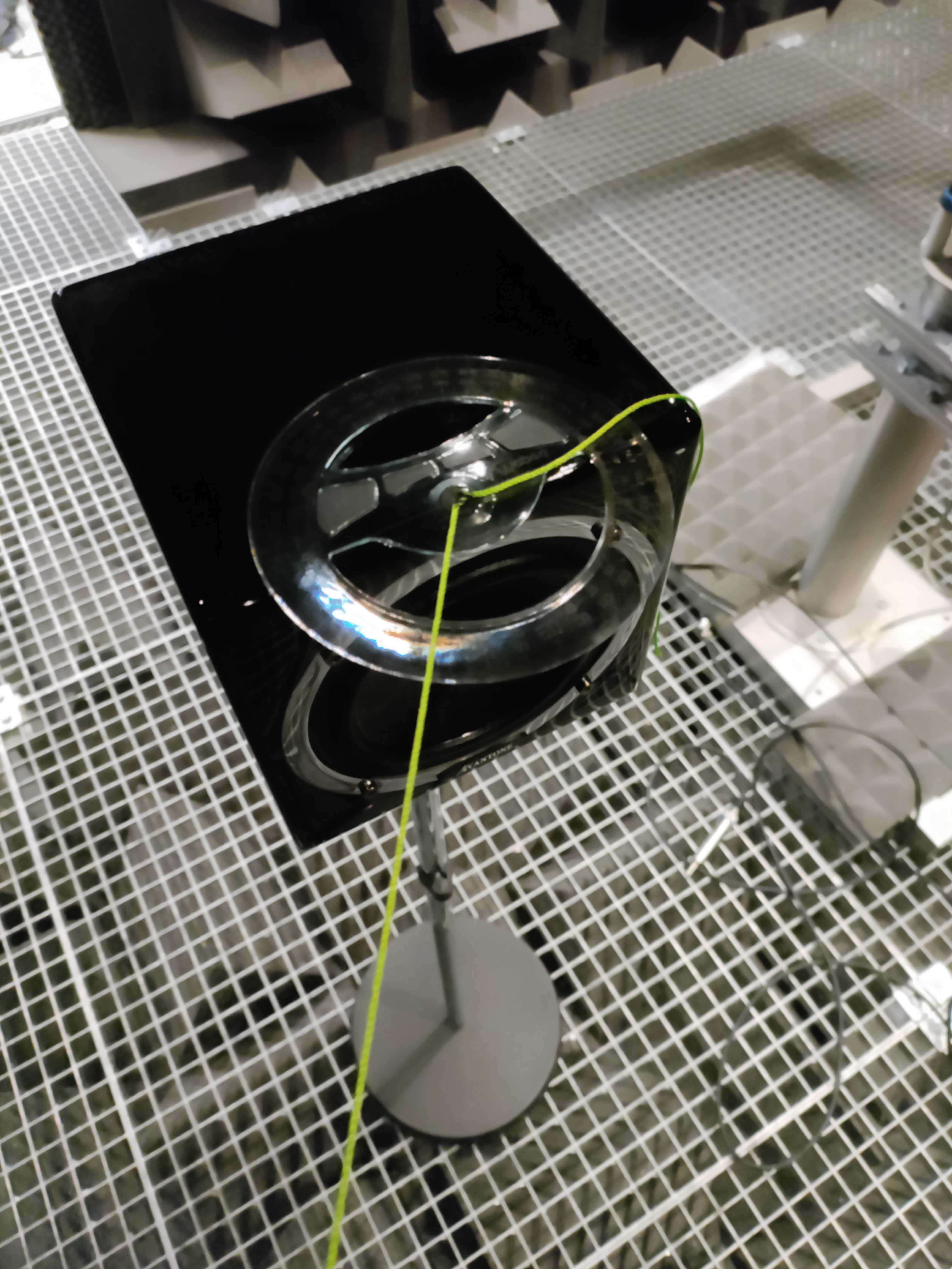
Figure 2: Photograph taken during the measurement of the Avantone MixCube.
We post-processed the measured impulse responses using on-axis source correction, dividing out the loudspeaker's own frequency response so that the results reflect the directivity pattern of the source, independent of its tonal character.
Simulation
To replicate anechoic conditions, we modeled a cubic room with 3-meter side-lengths for each loudspeaker. We assigned all interior surfaces idealized absorptive materials with a broadband absorption coefficient of 0.95, meaning 95% of incident sound energy is absorbed at each reflection, effectively simulating the near-total absorption of an anechoic chamber lining. We placed the source with its membrane center at the room center, surrounded by an array of mono receivers matching the configuration in Figure 1.
Despite the highly absorptive boundaries, trace reflections can remain in the simulated impulse responses. We applied time-windowing to isolate the direct sound arrival and remove these residuals, yielding perfectly anechoic responses. Figure 3 illustrates this process.
Example 1: Single-driver loudspeaker (Avantone MixCube)
The Avantone MixCube is a compact, single-driver monitor with a full-range cone driver. The driver cone is approximated as a rigid pulsating piston (a flat disc vibrating uniformly) mounted in the speaker's actual enclosure geometry, and we simulate it using the DG solver. The results show that this approximation captures the loudspeaker's directivity well enough for applied room acoustic simulations up to 11,000 Hz.
Simulation model
We created a boundary-velocity submodel of the Avantone MixCube using the following dimensions:
- Enclosure width, depth, and height: 0.165 m
- Membrane diameter: 0.08 m
- Membrane center height: 0.0825 m
We ran simulations up to 11,000 Hz. The resulting simulation definition is visualized in Figure 4.
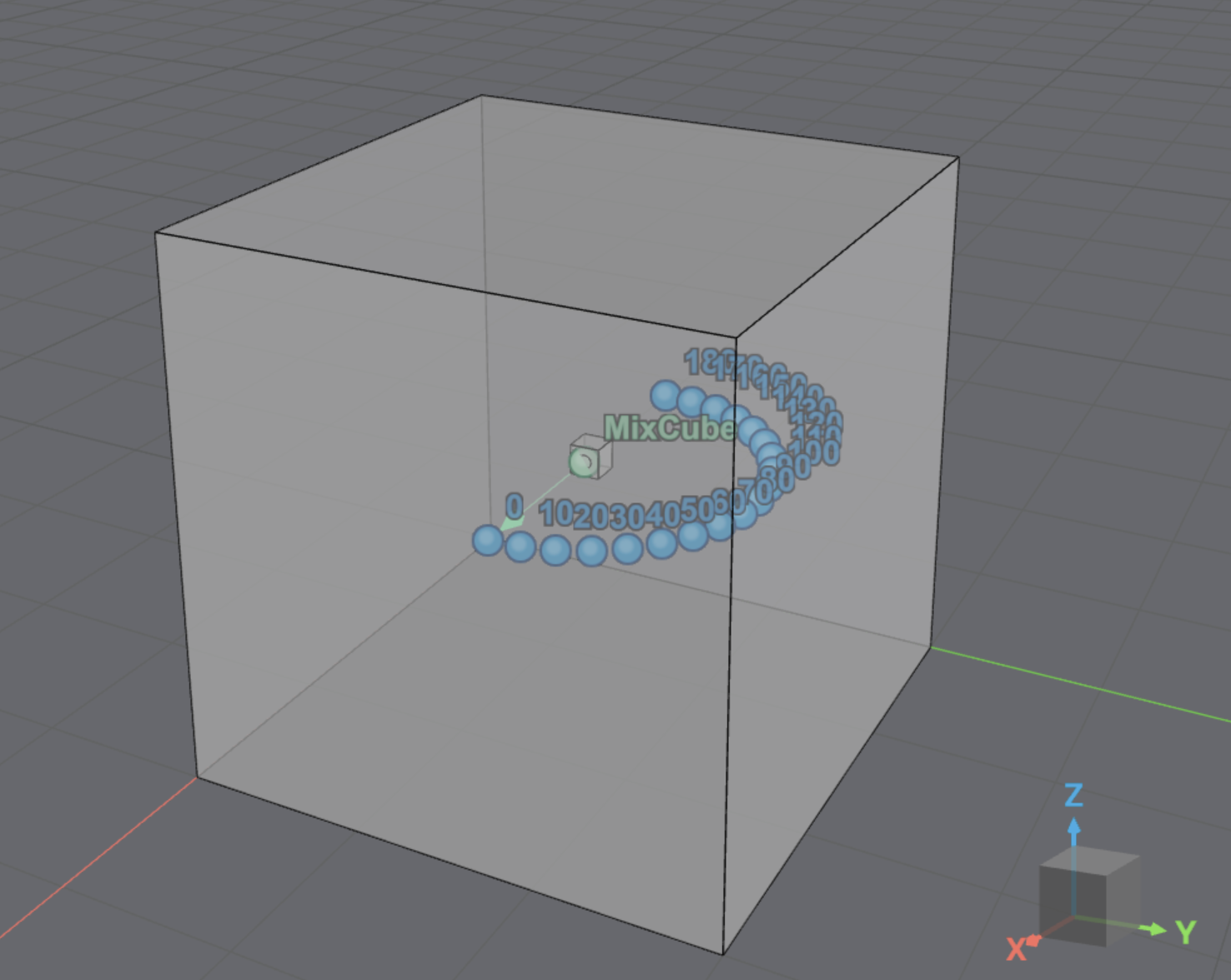
Figure 4: Overview of the Avantone MixCube simulation definition.
Results
Figure 5 compares simulated and measured polar patterns (plots of sound pressure level as a function of radiation direction) at several frequencies. A perfectly omnidirectional source would appear as a circle; a directional source produces a narrower lobe pointing along its forward axis.
The simulated responses agree well with measurements across the full frequency range. At 8 kHz, minor amplitude variations begin to appear, but the overall directivity shape is still well captured.
Figure 6 shows 1/3 octave band averaged frequency response comparisons at angles from 0° to 160° in 20° steps, giving a complementary view of how the simulated and measured responses agree across the full frequency range at each measurement angle.
The boundary-velocity submodel accurately reproduces the spatial response of the Avantone MixCube, capturing the scattering and diffraction that the loudspeaker enclosure introduces into the sound field. The single-piston approximation doesn't account for complex high-frequency effects such as membrane break-up modes, but it delivers good accuracy at low frequencies and reasonable performance at high frequencies.
Example 2: Two-way studio monitor (Yamaha H8)
The Yamaha H8 is a two-way studio monitor: it uses a woofer (large driver) for low frequencies and a tweeter (small driver) for high frequencies, each mounted on the same enclosure. This example extends the boundary-velocity submodel approach to this multi-driver configuration.
We compared two simulation strategies. In the fully wave-based simulation, we modeled both drivers using the DG solver. In the hybrid simulation, the woofer still uses the DG solver, but we modeled the tweeter using the GA solver. Because the tweeter operates at high frequencies, where sound wavelengths are short relative to the enclosure dimensions, the GA solver is well suited here, and the hybrid approach can reduce simulation cost while retaining accuracy where it matters most. This comparison helps clarify when a fully wave-based simulation is worth the additional computation.
Simulation model
We modeled the Yamaha H8 enclosure geometry directly in Rhino, tracing the enclosure shape and driver positions from manufacturer drawings. The woofer and tweeter membranes are each approximated as a rigid pulsating piston, as in the Avantone MixCube case study. Figures 7 and 8 show the resulting geometry models.
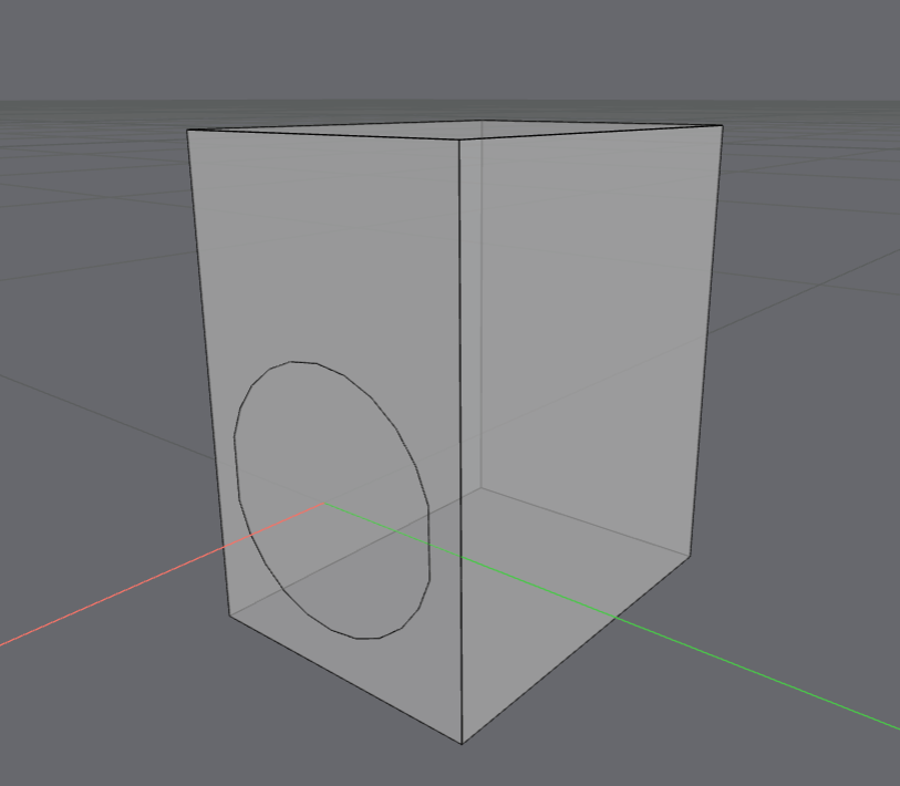
Figure 7: Geometry model of the Yamaha H8 woofer.
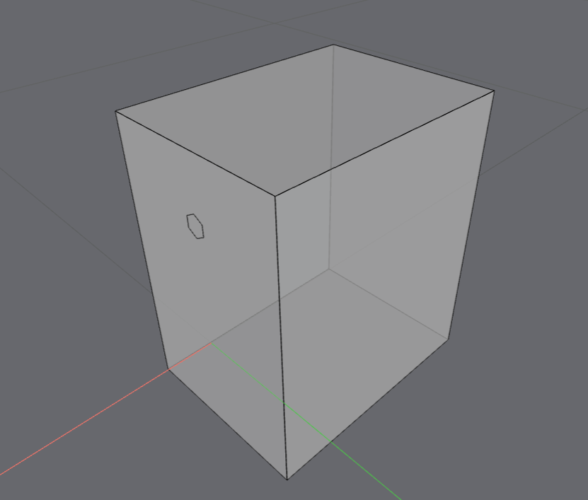
Figure 8: Geometry model of the Yamaha H8 tweeter.
Both the woofer and tweeter are injected as separate boundary-velocity submodels. The woofer is always solved using the DG solver (up to 2500 Hz); the two strategies differ only in how the tweeter is handled. In the fully wave-based simulation, the tweeter is also solved with the DG solver (up to 11,000 Hz). In the hybrid simulation, the tweeter is instead represented as a directive point source in the GA solver, with its directivity pattern derived from the free-field results.
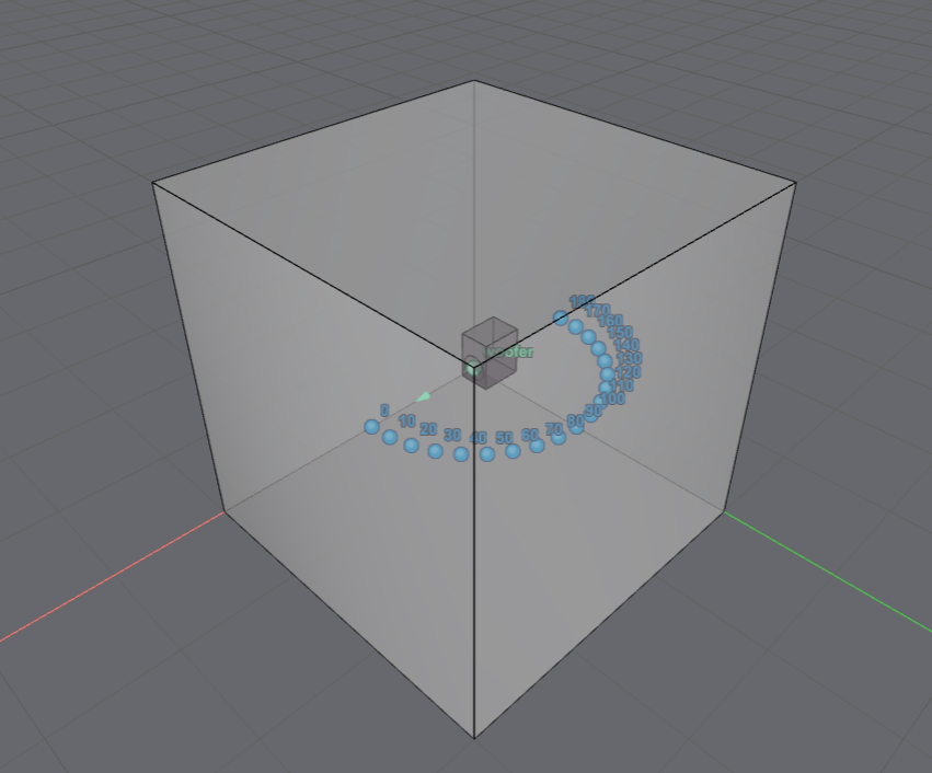
Figure 9: Simulation definition for the Yamaha H8 woofer.
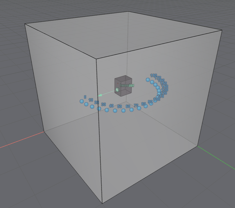
Figure 10: Simulation definition for the Yamaha H8 tweeter.
In post-processing, we apply a 2000 Hz crossover to the woofer and tweeter responses (third-order Butterworth low-pass and high-pass respectively), then sum the two bands to form a full-range impulse response. We also apply a time window around the direct sound arrival to suppress residual reflections from the room boundaries, as in the Avantone case study.
Results
Figure 11 compares the measured polar patterns against both the fully wave-based and hybrid simulations at several frequencies.
Figure 12 shows 1/3 octave band averaged frequency response comparisons at angles from 0° to 160° in 20° steps for both simulation strategies.
The boundary-velocity submodel reproduces the measured directivity of the Yamaha H8 well across the full frequency range. The fully wave-based and hybrid simulations are nearly identical, with only minor deviations at high frequencies.
Summary
Both case studies show that boundary-velocity submodels accurately reproduce loudspeaker directivity under anechoic conditions, for both single-driver and multi-driver configurations, and with both fully wave-based and hybrid simulation workflows.
For the Avantone MixCube, the DG solver captures the directivity well across the full simulated bandwidth, with only minor deviations at the highest frequencies.
For the Yamaha H8, both the fully wave-based and hybrid strategies agree closely with measurements, and the two strategies are nearly indistinguishable from each other. Under anechoic conditions this is expected: without objects in the sound field to introduce diffraction, scattering, or modal resonances at low frequencies, the GA solver is an accurate and computationally efficient choice for the tweeter. When injecting the source into a realistic room, a wave-based treatment of the woofer becomes more important, as low-frequency wave phenomena from the room geometry and its contents become significant.