Analyze Device

We do processing behind the scenes to convert discrete inputs (response from a finite selection of angles) to a continuous representation where we can compute the response from any angle. This is done using a spherical harmonics decomposition of the input data and for a varying degree of complexity of the input data, we need a varying degree of complexity of the spherical harmonics to capture the input. After a device is created and added to the device library, you can use a tool to analyze the device to ensure it captures the intended/expected behavior.

Device analysis widget

Assuming you have a DeviceObj object, you can run this:

device.plot()

If the widget loads with a white background, run the line above, and it should appear correctly. In this section, we'll go through the different parts of the widget and explain what information it provides.

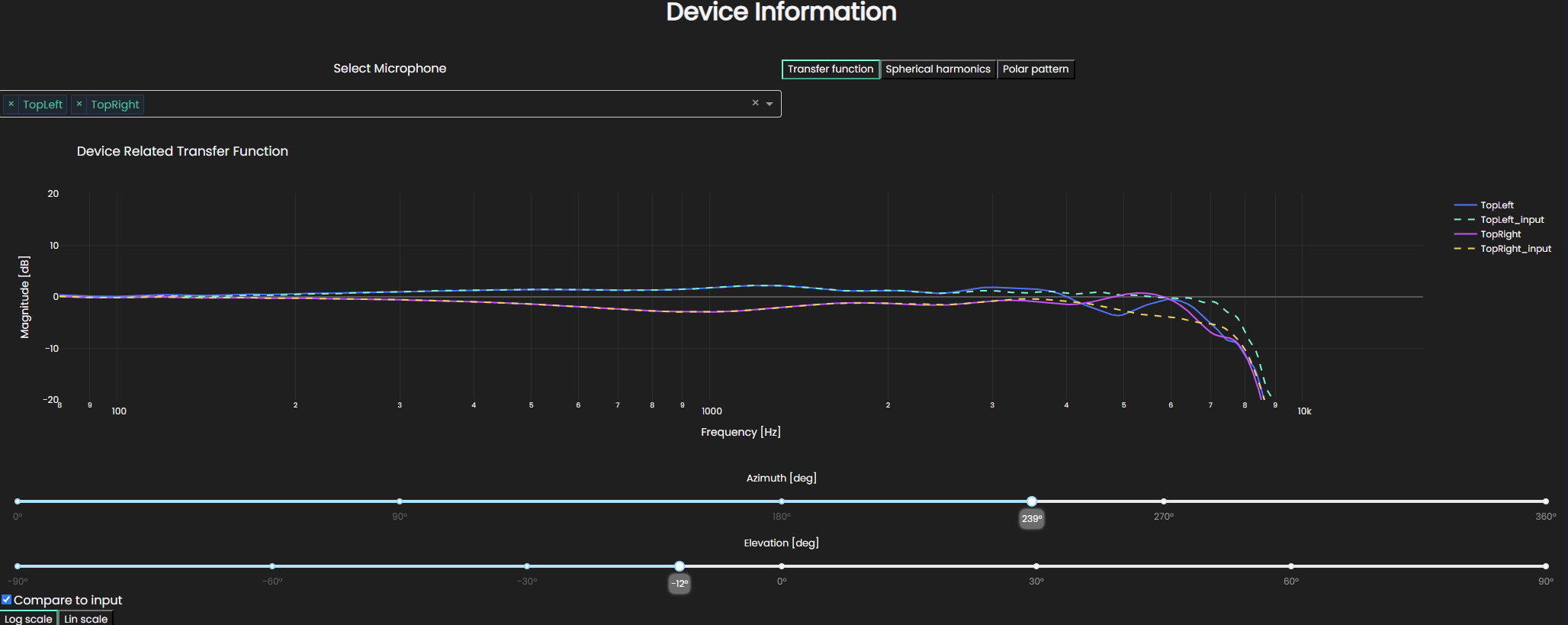
Transfer function

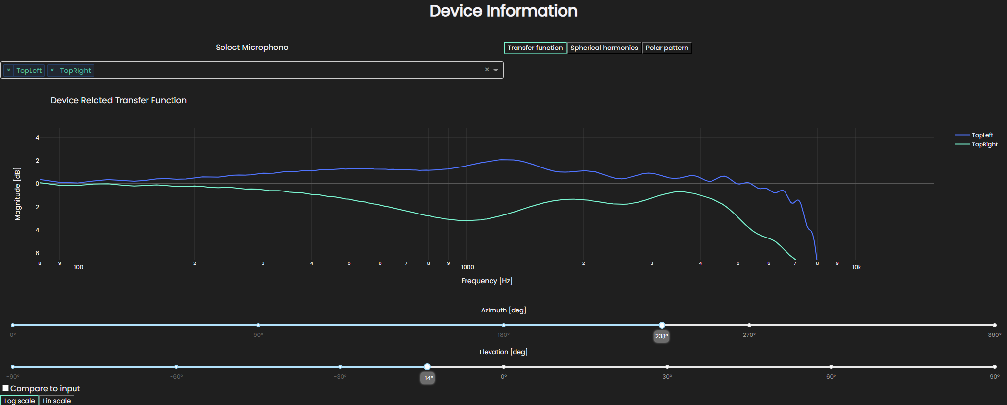
With the Transfer function plotting tool you can look at the response of the device for any direction as a function of frequency with either logarithmic or linear frequency axis. What is displayed is the transfer function computed from the spherical harmonics for the chosen microphones on the device. To investigate, up to which extent the spherical harmonics capture the input data, you can check the Compare to input check mark to plot the input transfer functions in a dashed line. The inputs are only available for selected angles, so this picks the closest angle to what you suggest and plots that.

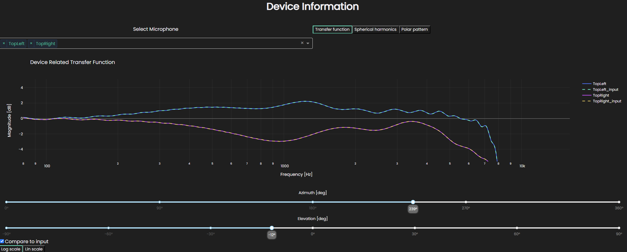
In the displayed case, the spherical harmonics capture the transfer functions perfectly.

Spherical harmonics

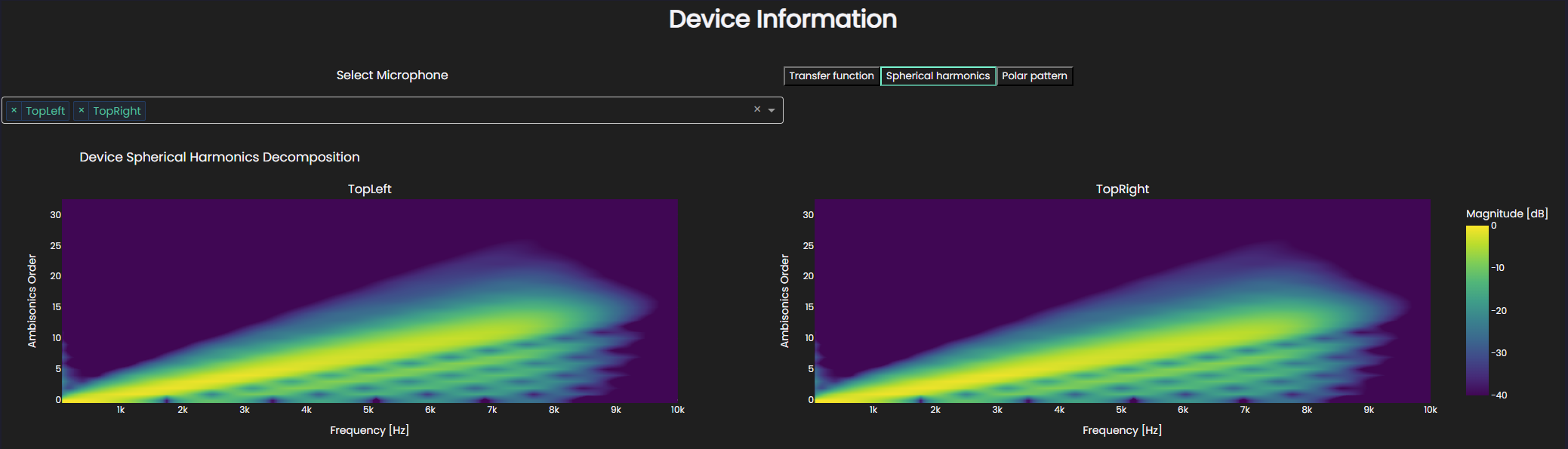
This shows how the energy in the of the microphone directivity is distributed in frequency and ambisonics order. The expected behavior here is that the brightest colors align linearly with a gradient which is controlled by the distance from origin of coordinate system to the microphone. In this particular plot, we also see some fainter colors above the line which relate to the energy which gets diffracted around the device. It can be seen in this plot, where the top of the plot is dark (meaning low energy), that we have a high enough ambisonics order to capture all the energy that we want to capture. This was also reflected in how well the input transfer functions were captured. On the other hand, if we render the same device at a lower ambisonics order, e.g. order 8, we can see that the energy at the top of the plot is still high, so we are not capturing all the energy we would want to.

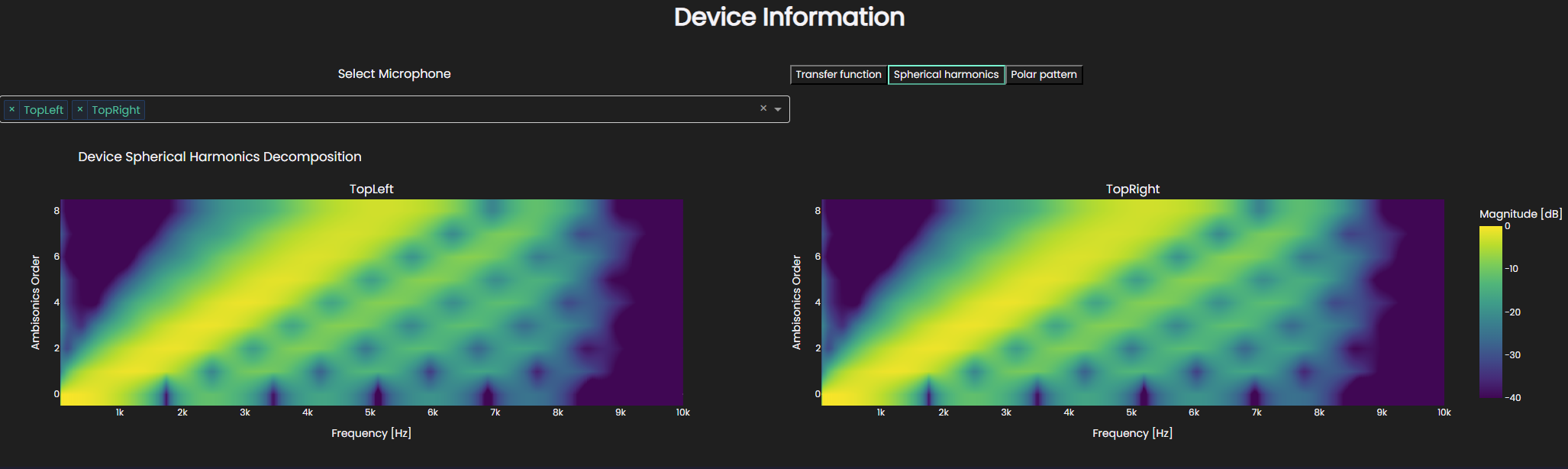
Which we can also see in how the transfer functions are captured, quite well for the lower frequencies, but much worse for the higher ones.

Polar Pattern

The widget also has the option of visualizing the directivity of the microphones in two-dimensional polar pattern for three different planes. The plot is created by computing the response for every angle along the respective plane for a certain frequency. The frequency slider is then used to look at the patterns at different frequencies.

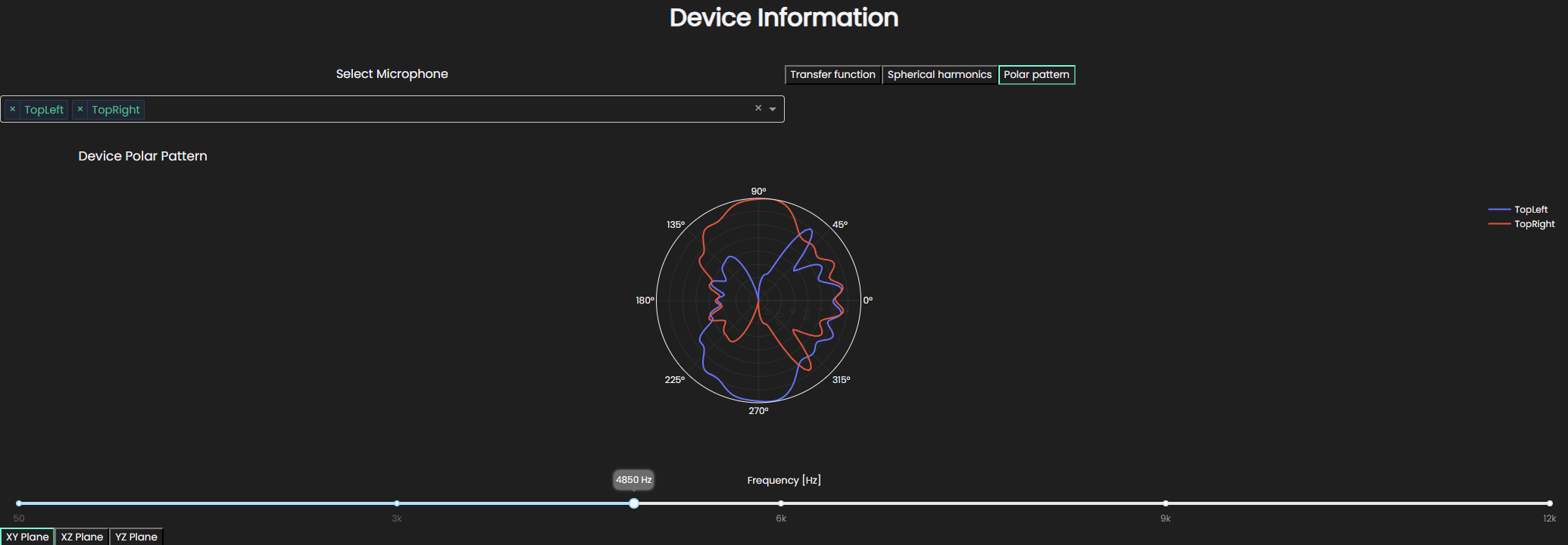
In this particular case, you can see that the microphones have responses which are mirrored around the center.

The created device can be imported in to simulation where there is a spatial receiver. This covered more in depth in our results section