Plotting

Overview plots

The Results class and it's associated acoustic parameter and impulse response classes come with a handful of plotting widgets to visualize results, both on a simulation level and on individual impulse response level. The plotting widgets are dynamic where you can zoom into specific parts of the plots and go back by double clicking. By clicking the legends you can show/hide individual traces and you can also save png files by clicking the camera icon which appears when you hover over the plot the your mouse.

As an instance of the Results class has been created, you can bring up the simulation overview widget like this:

# Get the results object for already downloaded results in `download_directory`
# This downloads into the directory if results are not found there.
results = get_results_object(download_directory)

# Start results plot widget
results.plot()

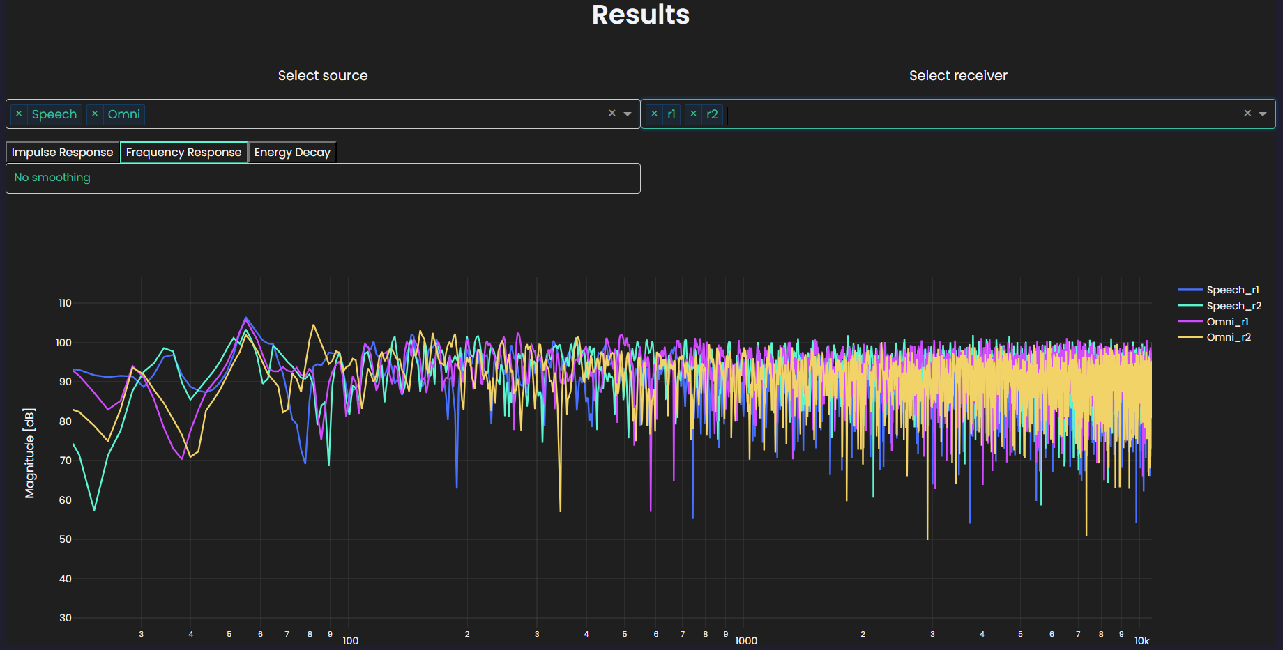
In this widget you can plot all the sources and receivers in the simulation simultaneously. You have access to impulse and frequency responses (which can be averaged with fractional octave bands) and energy decay curves for each octave band.

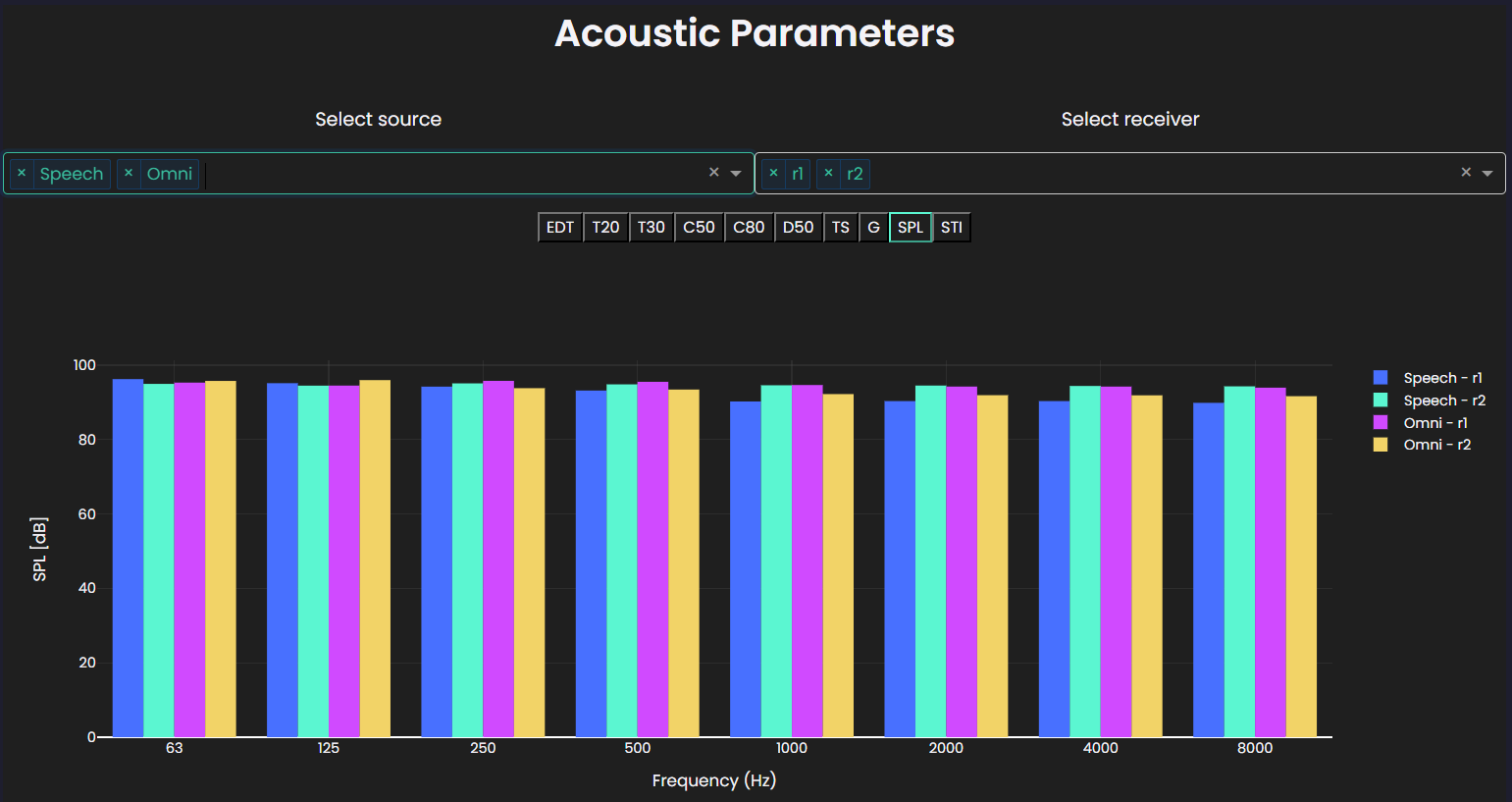
Similarly, there is a tool for viewing the acoustic paramters:

results.plot_acoustic_parameters()

Impulse response plots

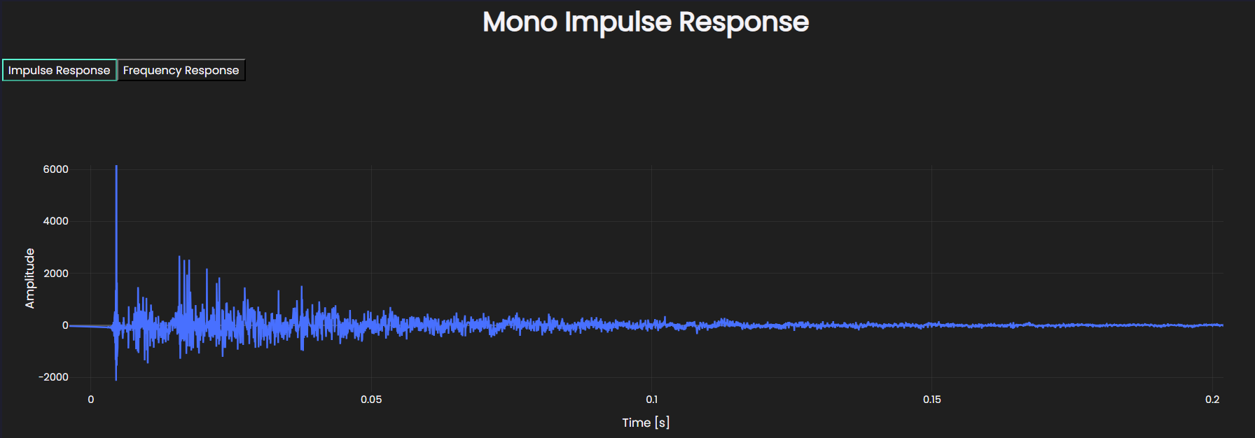
Similarly you can plot single impulse response object as such:

receiver = "r3"
source = "Omni"

mono_ir = results.get_mono_ir(source=source, receiver=receiver)

mono_ir.plot()

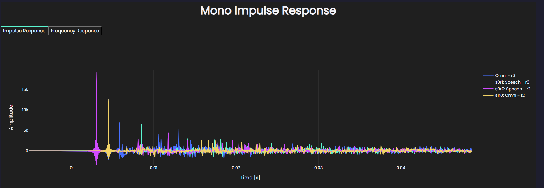
The impulse response plots (device and mono) also have an optional comparison field when you want to compare two or more receviers in a single plot. To do so, you pass a dictionary with the keys as names of the comparison cases and the values being the IR classes:

# Find a few comparison impulse responses
mono_ir2 = results.get_mono_ir(source="Speech", receiver="r3")
mono_ir3 = results.get_mono_ir(source="Speech", receiver="r2")
mono_ir4 = results.get_mono_ir(source="Omni", receiver="r2")

# Make a plot with each of those impulse responses in there
mono_ir.plot(comparison={"s0r1": mono_ir2, "s0r0": mono_ir3, "s1r0": mono_ir4})

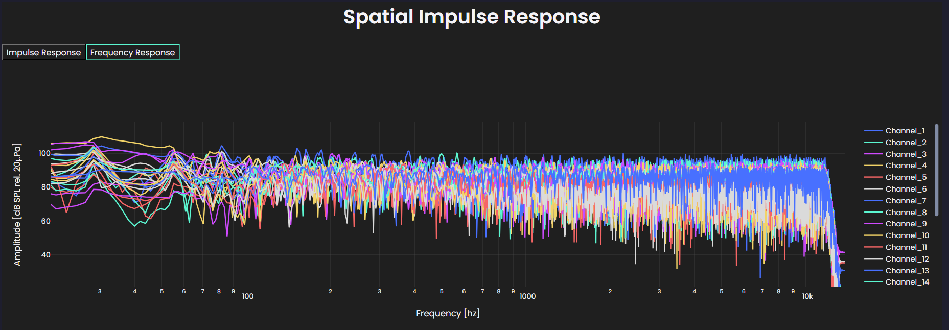
For spatial impulse responses, there is a limit to how many channels can be plotted at a time (64) as the plot widget becomes quite laggy when hundreds of traces are plotted at a time. The plot also quickly becomes quite crowded as can be seen here:

spatial_ir = a.get_spatial_ir(source="Omni", receiver="r3")
spatial_ir.plot(channel_range=(0, 24))

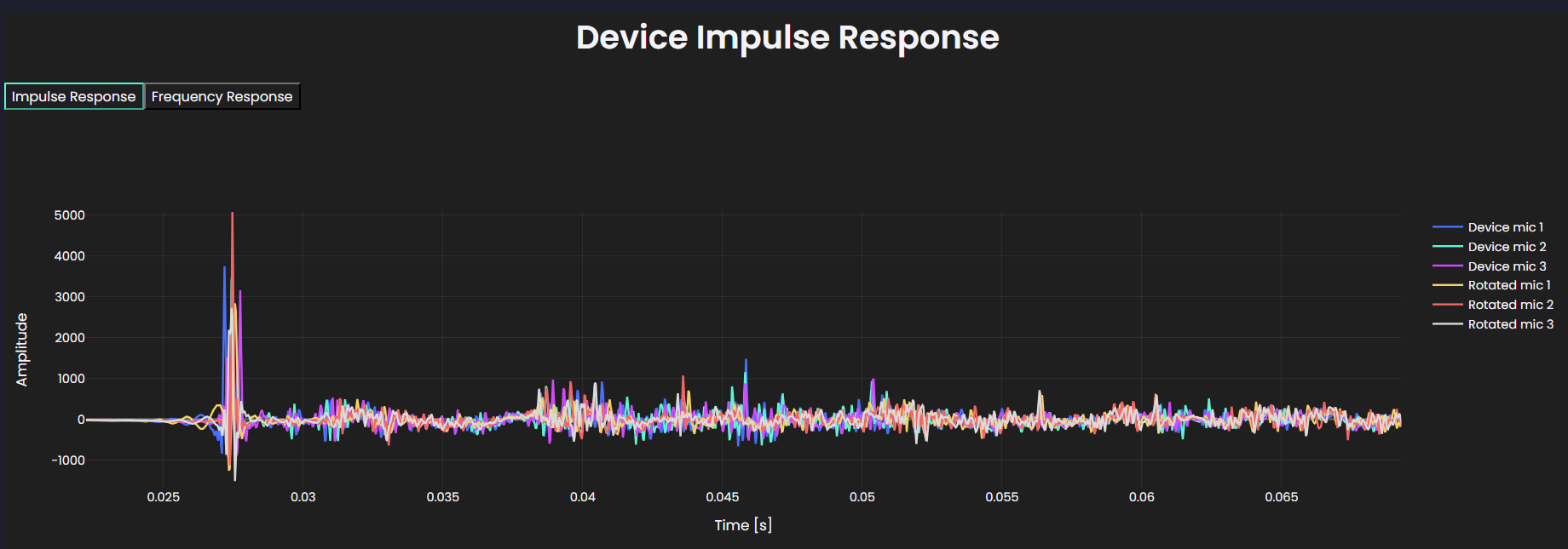
Similar to the monoIR comparison plots, a deviceIR plot will display the microphones on the device in a single plot. Other rendered devices can also be added to the same plot using the comparison argument.

# Render device from a spatial IR
device_ir = spatial_ir.render_device_ir(device=device)
# Render the same device, rotated 180 degrees in azimuth
rotated_device = spatial_ir.render_device_ir(device=device, orientation=treble.Rotation(180,0,0))
# Plot both renders in the same plot
device_ir.plot(comparison={"Rotated": rotated_device})