Tutorial: Reflection Tracking
This article provides a step-by-step tutorial for the reflection tracking view.
The simulation in this tutorial has already been set up and run so you don't have to do so again.
Overview
Reflection tracking is a visualization tool in Treble that shows the simulated image source paths, i.e. specularly reflected sound paths, between a source and a receiver.
Its primary purposes include:
- Optimizing the placement of acoustic treatment, i.e. absorbers or reflectors
- Optimizing the orientation of speakers
- Detecting unwanted reflections that may degrade listener experience
- Understanding the directionality of incoming reflections at a receiver point
- Analyzing how different surfaces affect the reflections
Note that Treble’s implementation of the image source method is pressure-based, which means it keeps track of reflected phase and the angle dependence of reflections (e.g. grazing incidence), making the results more physically faithful than purely energy-based methods.
Setup
In this tutorial we’re going to look at a concert hall and analyze the reflections between a selection of sources and receivers. An overview of the simulation setup is as follows:
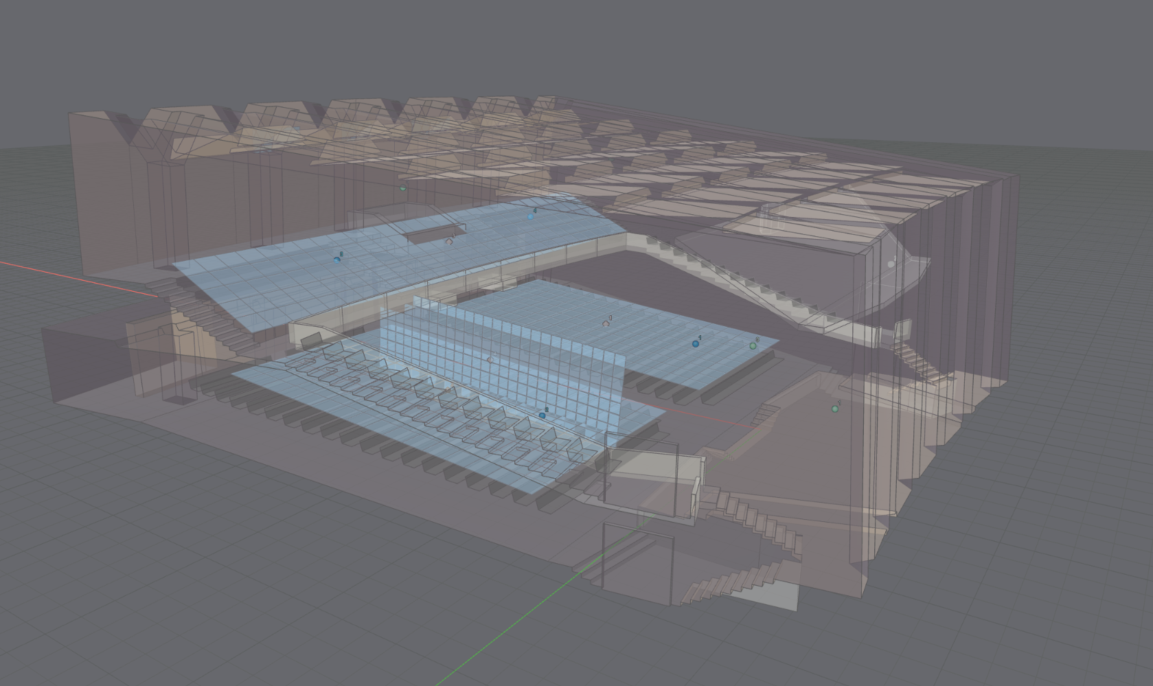
The model used in the simulation comes from the BRAS database. The materials and scattering values assigned to the surfaces in the room can be seen in the material section on the right:
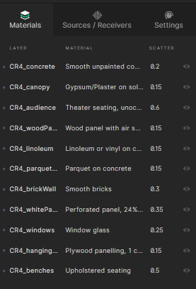
Selecting the Source/Receivers tab shows the sources used for the simulation, one omnidirectional source and four commercial speakers:
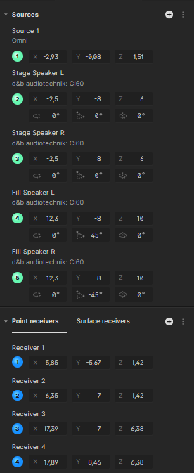
This simulation was run using only the geometrical acoustic solver. The image source order was set as third order. This means that all specular reflection paths that reflect of up to three surfaces are simulated and can be analyzed.
Interacting with the reflection tracking view
Select the results icon in the bottom right to analyze the simulation results:

The reflection tracking view can be selected from the top menu in the center:
![]()
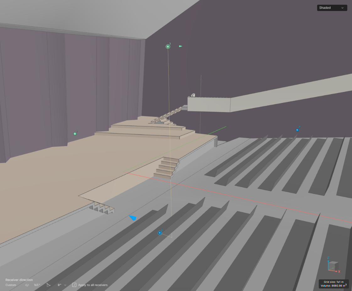
Your viewport should now look like this:
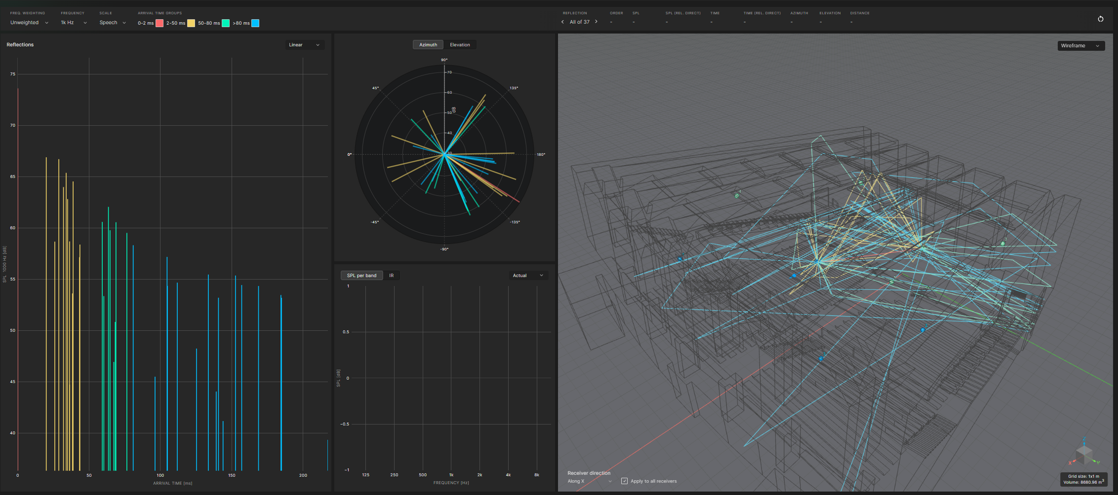
A detailed step-by-step guide of each component in the view can be found in our documentation. The following is a condensed overview of what can be found there. If you want to dive straight into an example analysis, head into the Analysis section.
Frequency weighting: In the top left of the view, the frequency weighting of the response can be chosen, it can be either unweighted, A-weighted or C-weighted.
Frequency: This dropdown is used to select between individual octave bands to analyze. The total level across all bands can also be displayed.
Scale selection and arrival time groups: The scale selector allows for the grouping of individual image source paths by arrival time, relative to the first reflection. There are three predefined groups to choose from. Individual segments of each group can be toggled on or off by selecting the colored checkboxes.
The information panel above the 3d viewport contains key information about the selected reflection. The ‘Reflection’ header is used to select between individual reflections. After a reflection has been chosen the panel shows some of its key properties such as the SPL, arrival time and arrival angle.
SPL graph: The largest graph in the view shows the sound pressure level of each reflection. The reflections are color coded based on their respective arrival time group. Each reflection can be selected on the graph. By doing so only the selected reflection path will be displayed in the 3d viewport on the right.
Azimuth and elevation: In this graph the angle of incidence of the incoming reflection in the horizontal plane (azimuth) and the vertical plane (elevation) are visualized.
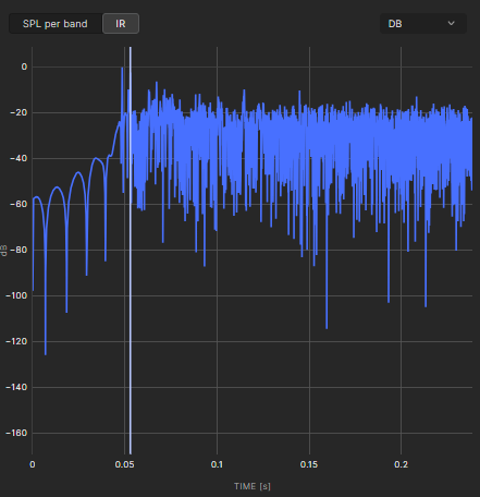
SPL per band and IR: This panel contains two options to get more information about the overall response: a. After selecting a reflection, the SPL per band view shows the SPL level of the chosen reflection across all octave bands. b. The IR view shows the simulated impulse response of the selected source receiver combination. The white line on the impulse response shows the time of arrival of the currently selected reflection.
There are two modes for the IR view. dB shows the IR in decibels, normalized by the pressure peak. Pressure shows the IR in Pascals.
The orientation of the receiver is shown with a blue arrow at the receiver position. The orientation can be edited in the bottom left corner of the viewport. Note that the selected orientation is only valid within the reflection tracking view and does not change the orientation of the receiver in the downloaded spatial IR, which is always along the positive x-axis.
You can change between sources and receivers and add other simulations to browse between in the simulation panel at the bottom.
Example analysis
To conclude the tutorial a brief example of how the reflection tracking view can be used to find unwanted reflection is given. Note that as previously stated this is only one of the use cases for the feature:
The default view shows all specular reflection paths from source 1 to receiver 1. From the SPL plot it can be seen that the decay is quite regular and controlled in the 1 kHz octave band:
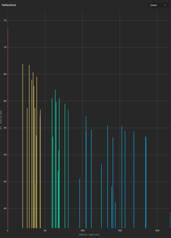
To analyze whether other sources in the model show the same behavior, select the third source ‘Stage Speaker R’ from the dropdown menu in the bottom left:

Looking at the SPL graph we can see that not long after the arrival of the direct sound (marked in red) there is a strong reflection that arrives at the receiver location (white). Selecting it on the plot will mark it white and show it on the impulse response and in the viewport:
Looking at the time of arrival we see that this reflection arrives approximately 53 milliseconds after the direct sound. We can also see that it’s only around 3.5 dB lower in magnitude.
In theory there is therefore a risk that this reflection might be perceived as an audible echo at the selected receiver location. However, since the reflection comes from the floor and reflects under the seating area this might not be problematic when an audience is present in the hall. This highlighting how important it is to analyze the spatial behavior of each reflection, not only the magnitude.
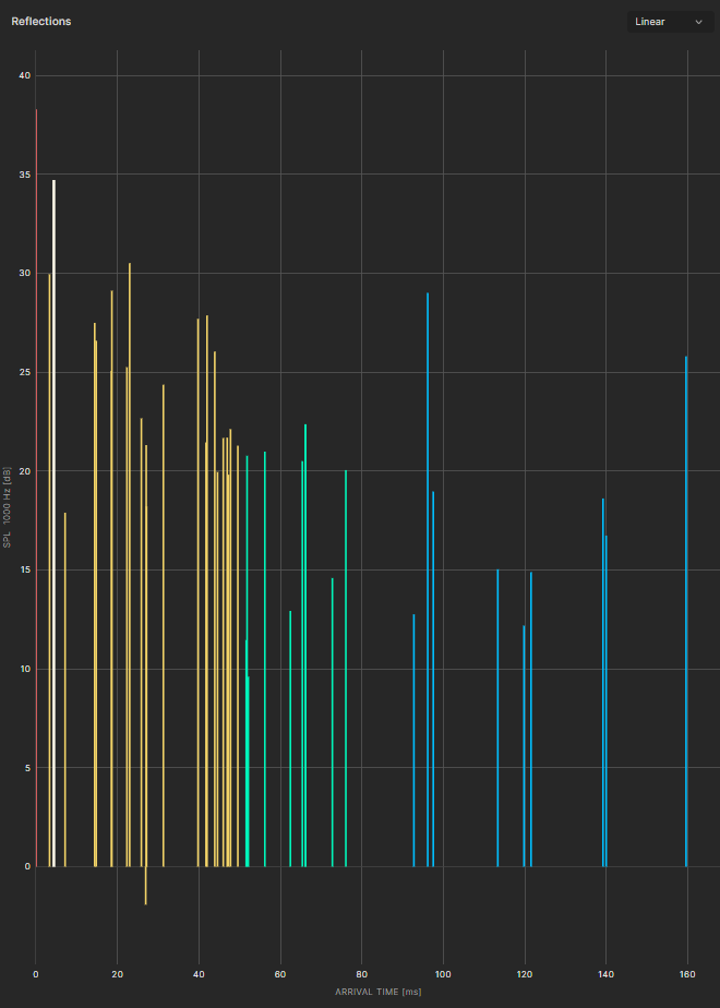
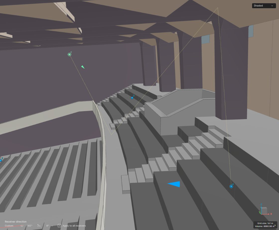
For another, and potentially more consequential reflection, select source 5 ‘Fill Speaker R’ and Receiver 4

On the SPL graph a strong reflection, rivaling the direct sound in magnitude can be detected (note that the selected loudspeaker is highly directive at 1kHz while also pointing away from the receiver). Selecting it on the graph reveals that it reflects of the floor and ceiling on its way from the source towards the receiver.
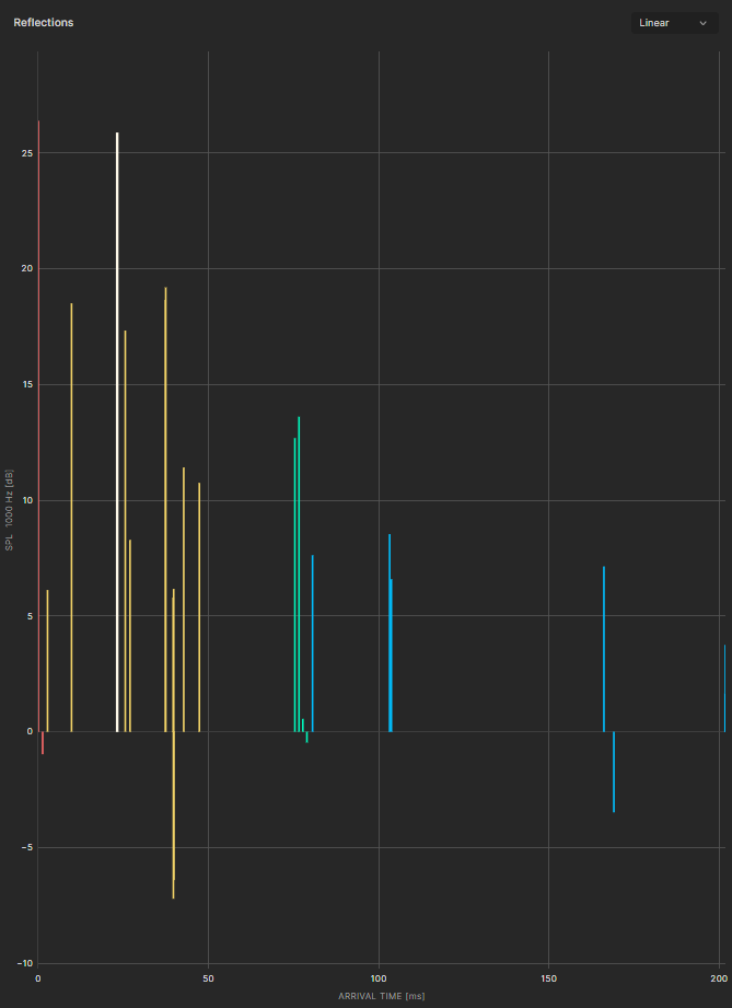
The reflection is also very apparent on the IR, as it’s only approximately 0.5 dB lower in magnitude than the direct sound, while arriving 75 milliseconds later. This highlights the need for treatment to counteract the disproportionate effect this reflection has on the impulse response. The most common ways to address the issue would be to increase the absorption of the ceiling, make the ceiling more diffuse or change the orientation of the speaker.
If you want to try to solve the issue, we encourage you to play around with the aforementioned settings and rerun the simulation to try and improve results.