Reflection tracking

The reflection tracking feature visualizes the image source paths in a simulation. By doing so it highlights some of the most relevant information that can be used to further enhance the acoustic design of a space. Example use cases include optimizing the placement of absorbers or reflectors, detecting reflections that distort the listener experience and analyzing the directionality of the sound at a receiver position.

tip

You can change the order of the image source method in the settings menu before running a simulation, under advanced settings. The order signifies how many reflections an image source path, from a source to a receiver, can take to be considered valid.

It's important to note that the implementation of the image source algorithm in Treble is pressure based, just like in our finite element wave solver. This approach brings distinctive advantages compared to other purely energy-based tools. The key advantages of our implementation are as follows:

1. The ability to store and account for reflected phase information. Our image source algorithm accurately calculates the reflected phase of an image source path as it reflects of a surface. Our impedance based material library has been specifically designed to take advantage of this, as the surface impedance can describe the changes in the magnitude and phase of a reflection at the surface of interest.
2. The reflection is dependent on the angle of incidence of an incoming wave. Our algorithm takes advantage of this as it allows us to factor in the angle dependency of the image source path as it hits a surface. This means that factors such as grazing incidence causing lower attenuation in general are factored into the calculations.

Read more about the image source method in Treble here. Details about the the contribution of the image source algorithm relative to the ray radiosity method can be found here. Note that in the reflection tracking view the scattering of a surface is taken into account, since the image source method only simulates the specular component of a reflection. The higher the scattering coefficient, the lower the contribution of the image source therefore becomes and vice versa.

Below is an image highlighting the different functions of the reflection tracking view, with further explanation for each one.

tip

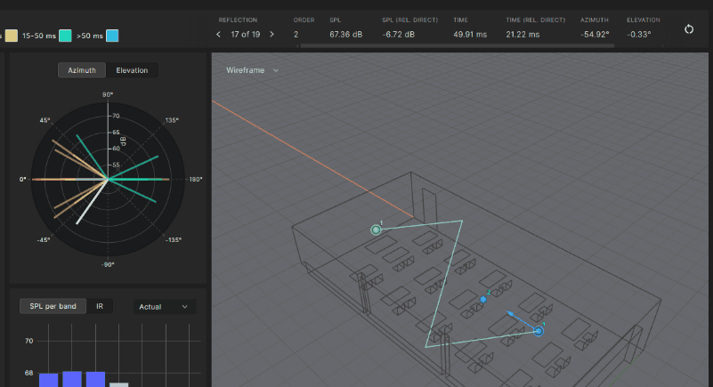
When going into the reflection tracking view all of the valid image source paths will be shown in the model.
To highlight a single reflection you can use the arrow keys on your keyboard, click on the arrows in the information panel (see number 4 in the image) or click on a reflection in one of the graphs.

1. Frequency weighting: Here you can decide the frequency weighting to use when analyzing results. There are three options to choose from:

   1. Unweighted, which is selected by default
   2. A-weighted
   3. C-weighted

2. Octave band selection: In this dropdown you can select between individual octave bands to analyze (125 Hz – 8 kHz). You can also view the total level across all bands by selecting Total. The total level is the summed sound pressure level of an individual reflection across all octave bands.

3. Scale selection and arrival time groups: The Scale dropdown lets you choose between three scales — Music, Speech and Studio — each of which defines its own set of arrival time groups (color-coded time ranges that group reflections by their arrival time relative to the direct sound). Once a scale is selected, the corresponding arrival time groups are shown as colored checkboxes below the dropdown. You can click a group checkbox to toggle it on or off, or double-click to isolate that group. The Scale you choose here also determines which reference-curve set is shown on the Reference curves view (available for Music or Speech).

4. The information panel: Contains key information about the selected reflection. The ‘Reflection’ control allows you to select between individual reflections (you can also use the arrow keys on your keyboard). After a reflection has been chosen the panel shows:

   • Order shows the image source order of the selected reflection, i.e. how many times it reflected off a surface before arriving at the receiver.
   • SPL is the sound pressure level of the selected reflection in dB
   • SPL (Rel. direct) is the sound pressure level of the selected reflection in dB relative to the direct sound
   • Time shows the time of arrival of the selected reflection in milliseconds
   • Time (Rel. direct) shows the time of arrival of the selected reflection in milliseconds relative to the direct sound
   • Azimuth and Elevation are the azimuth and elevation angles of the selected reflection at the receiver position, relative to the chosen receiver direction (see step 9)
   • Distance shows the distance the selected reflection has traveled within the geometry in meters.
   tip

   When viewing all reflections (i.e. no single reflection selected or filtering applied), three fields in the information panel become filter inputs: Order, SPL (Rel. direct), and Time (Rel. direct). You can enter a single value or a range (e.g. 1-3) to filter the displayed reflections. Whenever any filter is active — whether a single reflection is selected, a filter has been applied via these inputs, or a psychoacoustic zone is selected on the reference curves chart — a Reset all filters button appears, allowing you to revert all filters to their default settings and display all reflections again.

5. View tabs: These tabs allow you to switch between the default Reflection view and the Reference curves view. The Reflection view displays the SPL graph and reflection data as described above. The Reference curves view is described in detail below.

6. SPL graph: This graph shows the sound pressure level of each reflection plotted against its arrival time relative to the direct sound (the x-axis denotes arrival time in milliseconds, with the direct sound at 0). The reflections are color-coded based on their respective arrival time group. Clicking a point selects that reflection.

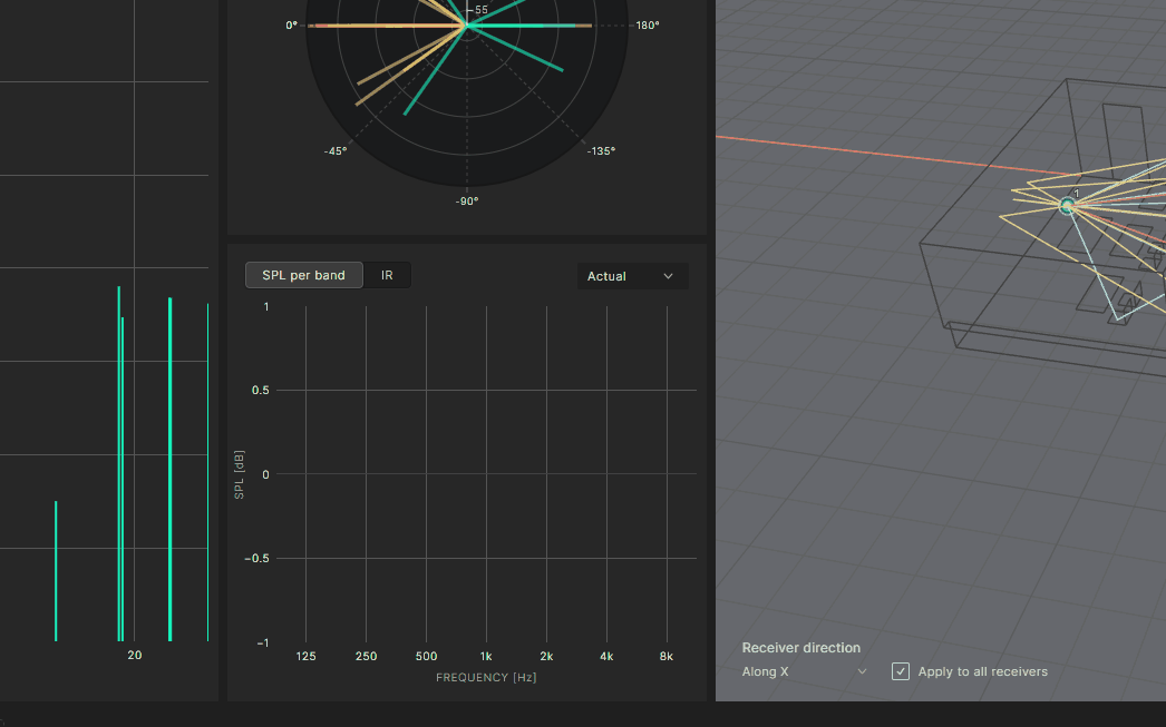
7. Azimuth and elevation: In this graph you can see the angle of incidence of the incoming reflection in the horizontal plane (azimuth) and the vertical plane (elevation). Keep in mind that you can change the receiver direction as explained in step 9, which will affect the angle of incidence relative to the listener direction.

tip

You can reorient the disc displaying the incoming angles by hovering over a degree number and dragging it. You can use this to orient the disc in the same manner as a receiver in the 3d model for easy reference.

8. Single reflection plots: This view contains two options to get more information about the overall response of a single reflection.

   1. After selecting a reflection the SPL per band view shows the frequency response of the chosen reflection across all octave bands. You can toggle between ‘Actual’ and ‘Rel. direct’ in the right corner. Actual shows the SPL level as is. Rel. direct shows the difference between the SPL level of the chosen reflection and the direct sound.

      You can also use this view to jump between the octave bands by selecting the bars in the plot.

   2. IR view shows the impulse response of the source receiver combination. Note that if the simulation is a hybrid simulation (combining the wave-solver and the geometrical acoustic solver) the IR shown is the hybrid IR. The IR can therefore contain more detail than can be inferred from the image source method the Reflection tracking view is based on. It is therefore mainly there for easy reference and comparison. The white line on the IR graph shows the time of arrival of the selected reflection on the SPL graph.

      There are two modes for the IR view. dB shows the IR in decibels, normalized by the pressure peak. Pressure shows the IR itself in Pascals.

      

9. All the valid reflection paths will be drawn in the 3d model. When selecting an individual reflection only that reflection will be drawn. The orientation of the receiver is shown with a blue arrow at the receiver position.

   You can change the orientation of a receiver from the Receiver direction control in the bottom left corner of the viewport. A dropdown offers the presets Along X, Along Y and Towards source, as well as a Custom option that exposes azimuth (0–360°) and elevation (-90–90°) inputs. Use the Apply to all receivers checkbox to set the direction for every receiver at once, or uncheck it to set the direction for the selected receiver only.

   

   note

   The orientation chosen is only valid within the reflection tracking view and does not change the orientation of the receiver in the downloaded spatial IR, which is always along the x-axis.

Reference curves

The reference curves view overlays environment-specific perceptual threshold curves on the reflection data, so individual reflections can be evaluated against established psychoacoustic criteria. Each reflection is plotted as a point — arrival time relative to the direct sound (in ms) on the x-axis against its sound pressure level on the y-axis — and the threshold curves, which are defined in dB relative to the direct sound, are overlaid on the same plot (shifted up by the direct-sound level so they line up with the absolute SPL of the reflections). The reflection points keep the same arrival-time-group coloring used elsewhere in the view.

note

On the Reference curves view the SPL is always shown unweighted and as a total across all bands, so the Frequency weighting and Octave band selectors (numbers 1 and 2) are disabled while this view is active.

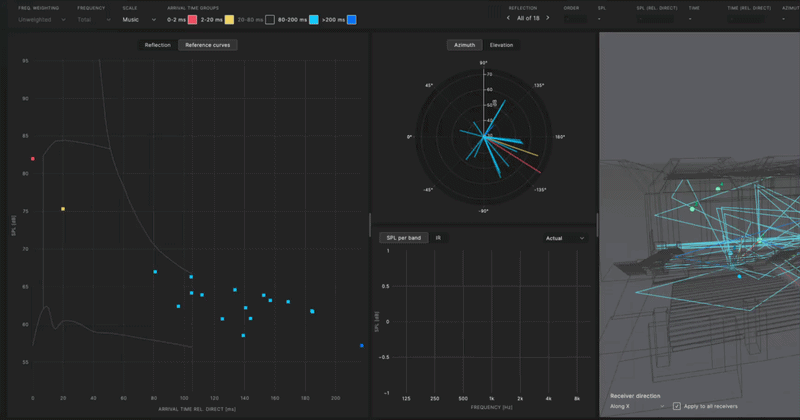
The reference curves are environment-specific. The acoustic environment is determined by the Scale selector (see number 3). The acoustic literature defines reference curves for two environments:

• Speech — applies a stricter set of threshold curves that reflect the higher sensitivity of speech to late reflections. Reflections exceeding the echo threshold at a given delay may degrade speech intelligibility or be perceived as distinct echoes. This is suitable for classrooms, lecture halls, conference rooms, and other spaces primarily used for spoken word.
• Music — applies more tolerant threshold curves, reflecting the fact that listeners are generally less sensitive to strong individual reflections during musical performances. Early reflections can enhance spatial impression and a sense of envelopment. This is appropriate for concert halls, rehearsal rooms, recording studios, and similar music-oriented environments.

The chart is divided into perceptual zones by three boundary curves (an audibility threshold, a sound-image / disturbance boundary, and an echo / image-shift threshold). Reflections below the lowest (audibility) curve are generally inaudible. Reflections that fall above the top curve — particularly those arriving well after the direct sound — should be examined more closely, as they may be perceived as echoes or coloration. Hovering over a zone shows its label, and clicking a zone filters the displayed reflections to those falling within it. You can use the reference curves in combination with the arrival time groups (see number 3 above) to systematically identify and address problematic reflections in your design.

The Speech reference curves are digitized from the reflection-level vs. reflection-delay figure in the Master Handbook of Acoustics [1]. The Music reference curves are digitized from Barron's diagram of the subjective effects of a single side reflection with music [2].

---

References

[1] F. A. Everest and K. C. Pohlmann. Master Handbook of Acoustics. McGraw-Hill Education, 6th edition, 2015.

[2] M. Barron. The Subjective Effects of First Reflections in Concert Halls — The Need for Lateral Reflections. J. Sound Vib., 15(4):475–494, 1971.