Surface receivers view
When selecting the Surface Receiver icon, you enter the Surface receivers view. Within this view, there are two distinct viewing modes: Acoustical parameters and Forced modal analysis.

Acoustical parameters
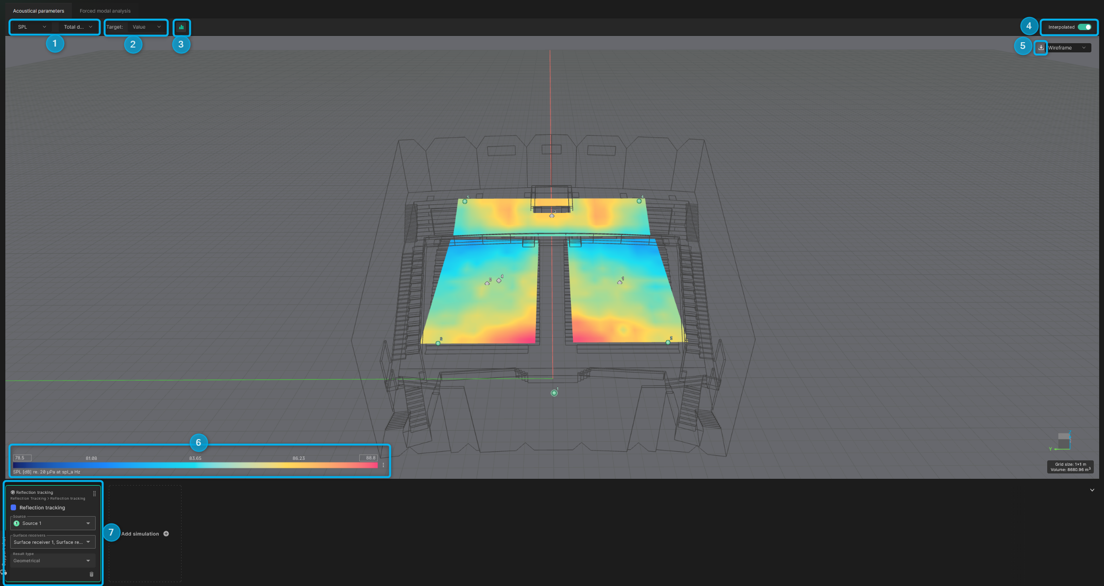
By default, the Acoustical parameters view is selected. This view shows a heatmap of all the acoustical parameters over the defined surface receivers in a simulation. The results are averaged over each octave band.
Below is an image highlighting the different functions of the Acoustical parameters view, with further explanation for each one:
-
You can toggle between the different acoustical parameters and octave bands to be displayed, using the highlighted dropdown menus. For some parameters broadband results can also be analyzed.
-
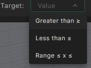
The target functionality allows you to analyze the spatial distribution of a parameter, with regards to a specific reference point or interval. After selecting the dropdown, you can choose whether you want to analyze the area where the parameter is above, below, or within a certain range.
Once selected, a new input field appears where you can input the desired reference value and analyze the area meeting the specified condition. The Target area percentage is based on the combined area of the selected surface receivers and factors in the area of each grid point.
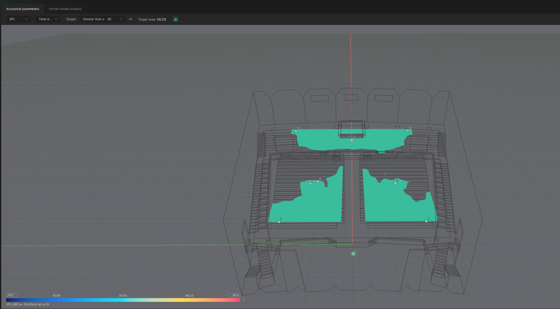
To return to the colored heatmap, select the  icon next to the Target area information panel.
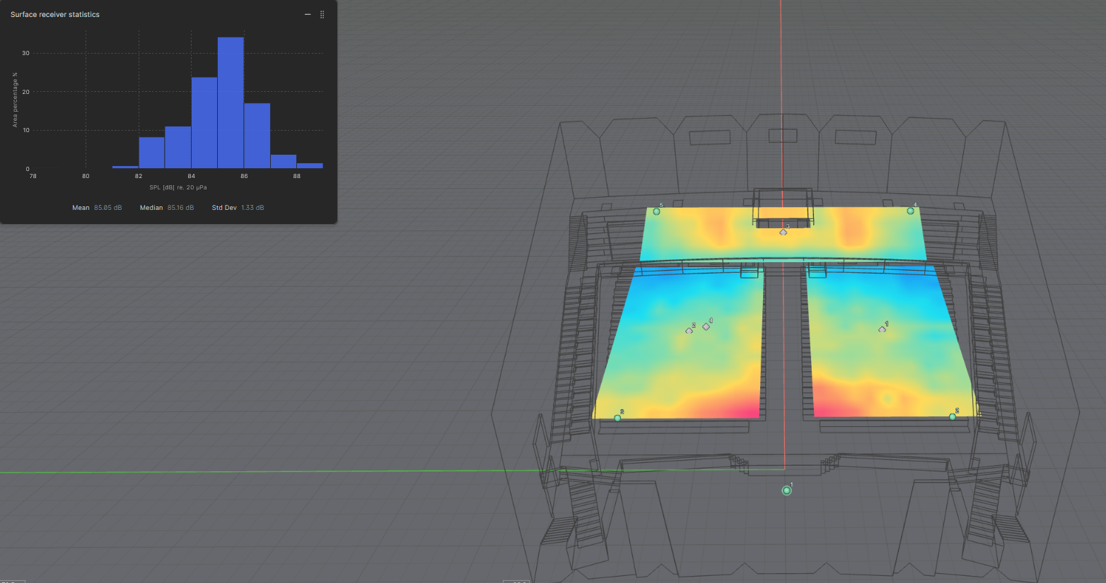
- The statistical information button provides spatial distribution information across the selected surface receivers. The field shows parameter value distribution along with the mean, median and standard deviation of the selected parameter, across the selected surface receivers, for the chosen octave band or broadband where applicable. The calculations factor in the total area of the selected surface receivers, along with the area of each individual grid point.
-
The default view for heatmaps is the interpolated view. This view uses bilinear interpolation to estimate the values between the center of each square to draw the color gradient along the surface. When disabling the interpolation, the heatmap shows each square with one color. The color shows the acoustic parameter value from the receiver in the middle of the square.
-
Using the export button, you can save the heatmap as a .png file with a white background and a centered legend. The file is generated according to the viewport's current orientation.
-
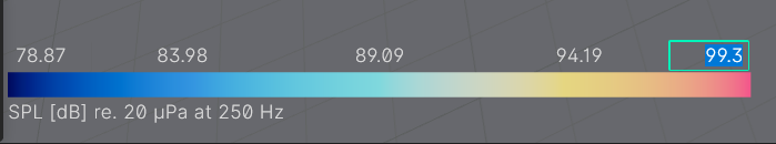
The legend of the heatmap is in the bottom left corner. Maximum and minimum values are auto-assigned based on the data being displayed. You can change the maximum and minimum values of the color bar by clicking the respective fields and inputting your desired value. This also fixes the values when comparing across different simulations.
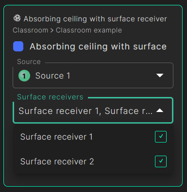
- The selection window allows you to choose which surface receivers to display. If multiple surface receivers exist, they are selected by default. You can toggle individual receivers on or off using the Surface Receiver dropdown.
Forced Modal Analysis
In this view you can analyze the spatial distribution of the frequency response for the selected source. The analysis can be conducted both for an individual source and summed sources.
The data being displayed in the heatmap is the magnitude of the wave based frequency response of each surface receiver grid for the chosen frequency. You can therefore use it to analyze how the chosen source interacts with and excites the room, with wave based behavior and reflected phase information taken into account. For that reason the feature is only enabled in the frequency range of the wave solver for the chosen simulation.
The name Forced modal analysis stems from the fact it’s based on the frequency response resulting from a particular source or sources. In other words the sources therefore “force” or “drive” the response.
Below is an image highlighting the different functions of the Forced modal analysis view, with further explanations:
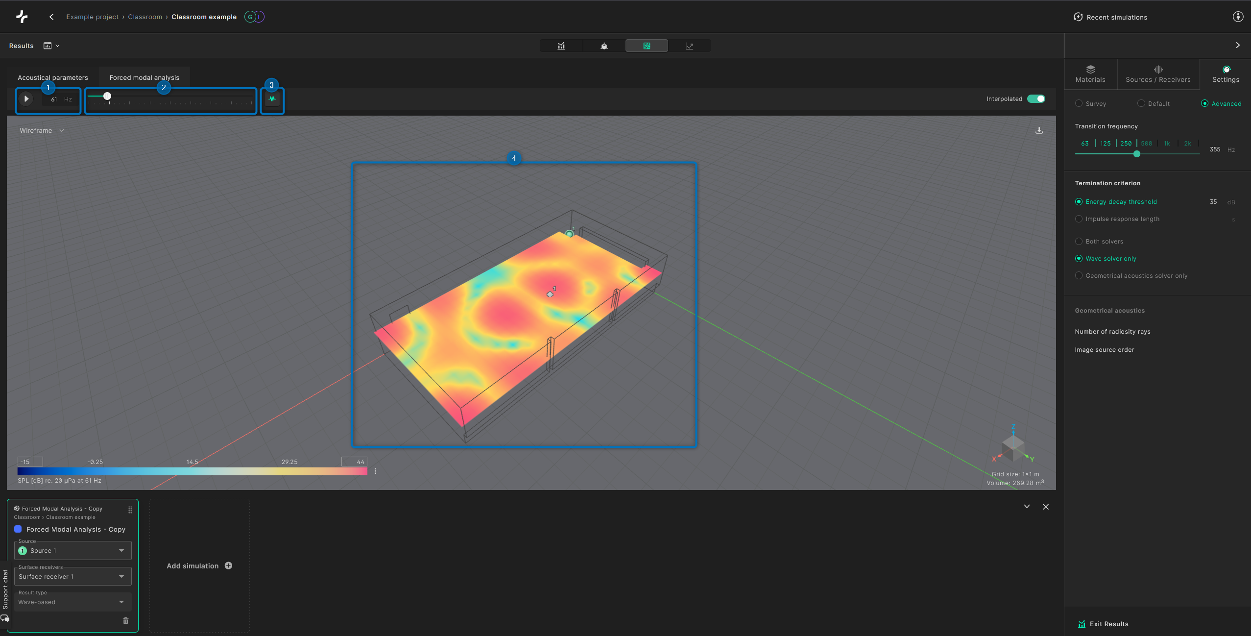
-
Using the input field, you can type or cycle through the frequencies to analyze. The play button automatically cycles through them.
-
The slider provides a quick way to navigate the frequency range by dragging it.
-
Clicking on the frequency response plot icon opens a new window displaying the frequency response for a selected point on the heatmap. If no point is selected, a message prompts you to do so.
You can click on the heatmap to select a grid point and view the frequency response plot for that location.
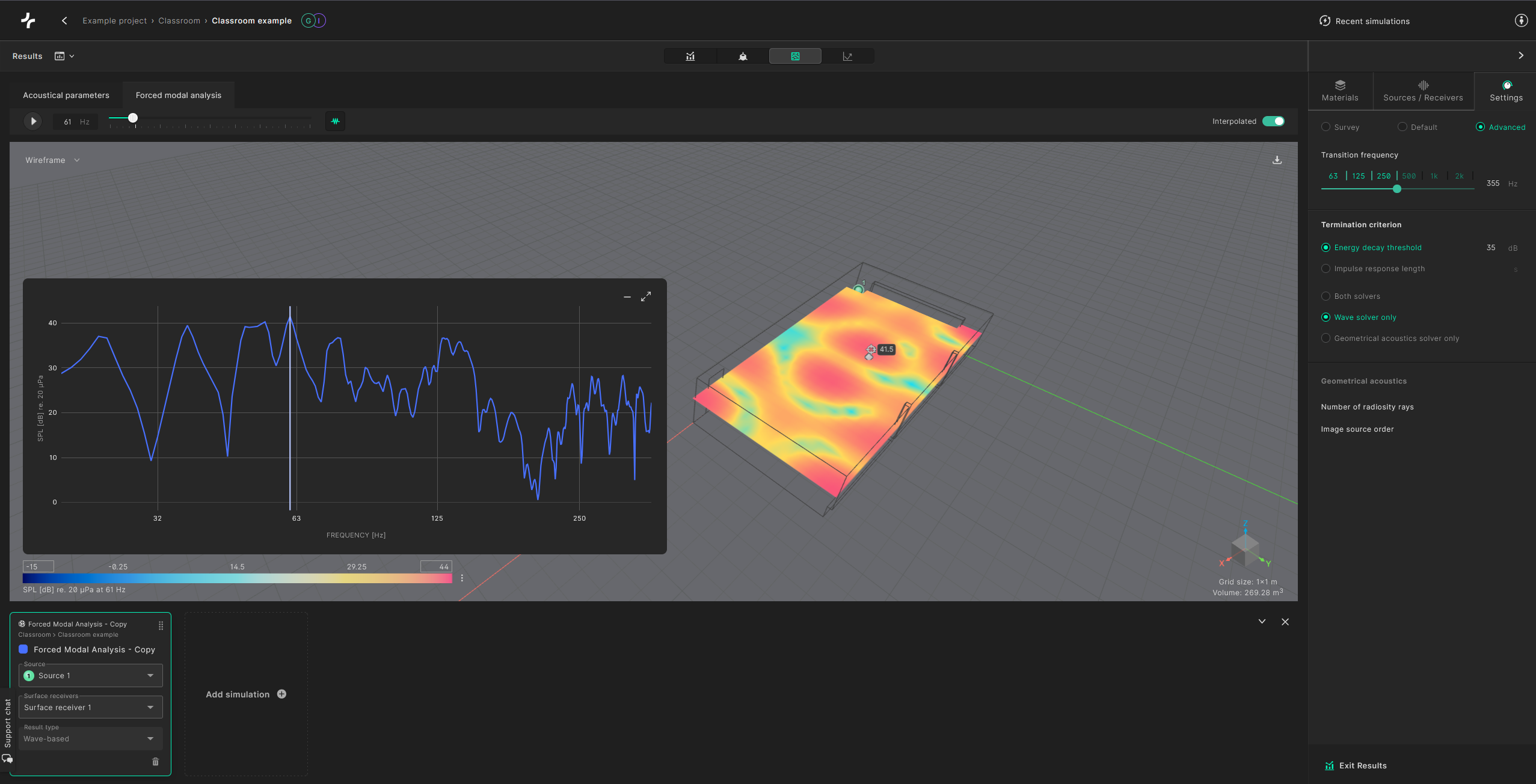
The white vertical line on the frequency response plot represents the currently selected frequency.
You can also navigate frequencies directly using the frequency response plot by selecting a point on the graph. The heatmap will automatically update.
The wave-based solver processes material input down to 50 Hz. Between 20–50 Hz, the results rely on extrapolated material data.
The other components of the Forced modal analysis view, such as the legend, exporter, and source selector, follow the same logic as described in the Acoustical parameters view.