Loudspeaker Modeling using Boundary-velocity Submodels

Introduction and Background

This article validates the boundary-velocity submodel feature of the Treble SDK using wave-based (DG-FEM) simulations up to 12,000 Hz. This method effectively models a loudspeaker as a rigid pulsating piston with an arbitrarily shaped enclosure.

We perform validation by comparing simulated and measured responses of a commercial single-driver loudspeaker (Avantone MixCube) under anechoic conditions, at different azimuth angles at a radial distance of 1 meter.

We show that the directivity of this loudspeaker is captured well enough for applied room acoustic simulations. Some dips or peaks are not accurately captured, most noticeably at high frequencies after around 5kHz, as seen in Figure 4. This is due to the single piston approximation.

Boundary-velocity submodels

Boundary velocity submodels are a feature of the Treble SDK that automate source injection in wave-based or hybrid simulations by embedding the source's geometry into the simulation, allowing flexible source placement within models. They rely on pre-computed results from free-field simulations.

A boundary velocity submodel provides an easily reusable sound source that is automatically source-corrected via a special correction filter derived from its corresponding free-field simulation. This filter normalizes the source’s frequency response to a flat 1 Pa on-axis at 1 meter under anechoic/free-field conditions.

When used in wave-based simulations, these submodels automatically apply the appropriate boundary conditions and mesh settings, ensuring accurate modeling of diffraction and other acoustic effects caused by the source's geometry.

If opting for a hybrid modeling approach, the geometrical acoustics part of the simulation uses a directive point-source with a directivity pattern derived from the free-field results. However, this study focuses exclusively on wave-based simulations. For full technical details, refer to the complete documentation.

Experimental Setup

This experiment consists of two parts: measuring and simulating the acoustic behavior of an Avantone MixCube loudspeaker under anechoic conditions.

The loudspeaker is positioned at the center of the room, with a semicircular array of 19 receivers arranged at 10° intervals along a 1-meter radius arc. The array spans from 0° to 180° in the counter-clockwise direction, using the loudspeaker's forward axis as the 0° reference. This configuration is illustrated in Figure 1.

Figure 1: Sketch of the source-receiver configuration used in both measurement and simulation setups, seen through a birds-eye view.

Measurement

Measurements were conducted in a semi-anechoic chamber using the source-receiver configuration illustrated in Figure 1. Impulse responses were measured using a swept sine method with a 10-second logarithmic sine sweep ranging from 50 Hz to 20 kHz. A GRAS 1/2'' free field microphone was used to capture the responses at each receiver position, with 24-bit/48 kHz sampling. To determine the measurement positions, a combination of a 1 meter long string and a protractor was used, see Figure 2.

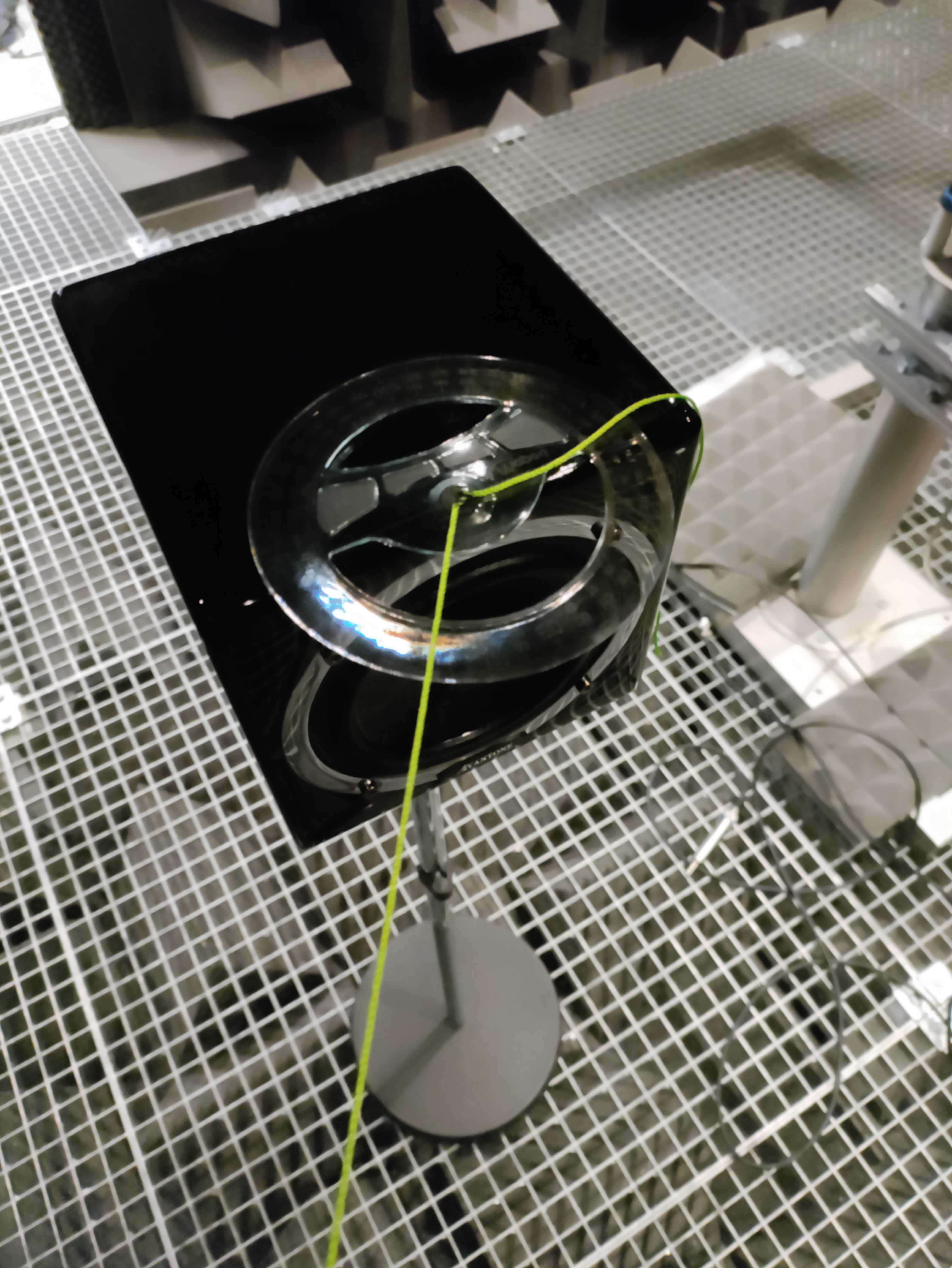
Figure 2: Photograph taken during the measurement of the Avantone MixCube.

To ensure consistency with the simulated impulse responses, post-processing on the measured impulse responses was performed using on-axis source correction. This step compensates for the inherent frequency-response of the loudspeaker, ensuring a meaningful comparison between measured and simulated data. The final impulse responses reflect the loudspeaker as if it has a flat on-axis response in anechoic conditions.

Simulation

To simulate anechoic conditions, a cubic room with 3 meter side-lengths was modeled. A boundary-velocity submodel of the Avantone MixCube was created using the dimensions:

• Enclosure width, depth, and height: 0.165 m,
• Membrane diameter: 0.08 m,
• Membrane center height: 0.0825 m.

The submodel source was positioned so that the center of its membrane aligned with the center of the room and surrounded by an array of mono receivers in the configuration as illustrated in Figure 1.

All interior surfaces were assigned idealized materials with a broadband absorption coefficient of 0.95. Simulations were performed up to 12,000 Hz, yielding valid impulse responses for each source-receiver pair up to this frequency. The resulting simulation definition is visualized in Figure 3.

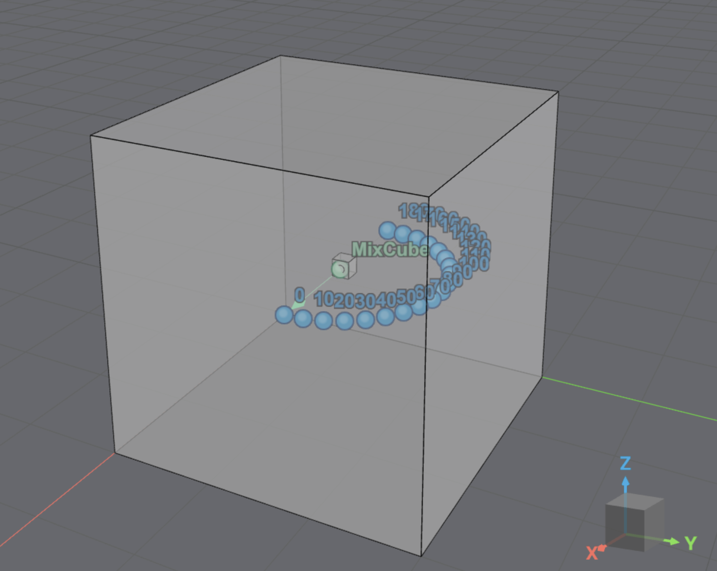
Figure 3: Overview of the simulation definition.

To suppress any residual reflections present in the impulse response, a time-windowing technique was applied, effectively resulting in perfectly anechoic impulse responses.

Results

Figure 4 presents a comparison between simulated and measured polar patterns at different frequencies. This allows for the assessment of how well the boundary-velocity submodel technique captures the directionality and overall magnitude response of the Avantone MixCube. From the polar plots we observe that the simulated responses show good overall agreement with the measured data, even at high frequencies there is a good match. In the 8 kHz plot we start to see minor variations in magnitude while the shape is still preserved.

Figure 4: Polar patterns

Conclusion

We have presented a case study of modeling an Avantone MixCube via the Boundary-velocity submodel feature of the Treble SDK, comparing simulated and measured data.

The results indicate that this feature provides a feasible means of approximating the actual spatial response of the loudspeaker, while accounting for scattering and diffraction effects caused by the loudspeaker’s presence in the sound-field.

While the simplicity of this method cannot capture complex phenomena at high frequencies (for example, the breakup-modes of the membrane). This provides a quick and simple way of modeling the main spatial response of this loudspeaker, with good precision at low frequencies, with reasonable high-frequency performance.