Mesh sizing in Treble SDK

In the Treble SDK, meshing is optimized for computational efficiency. Nevertheless, in some cases it might be needed to change the way in which certain parts are meshed. Think of a source, where a membrane is moving, or the placement of a virtual microphone as small as possible to simulate the DRTF.

In the following examples we show how it is possible to alter the automatic mesh optimization.

Simplification threshold

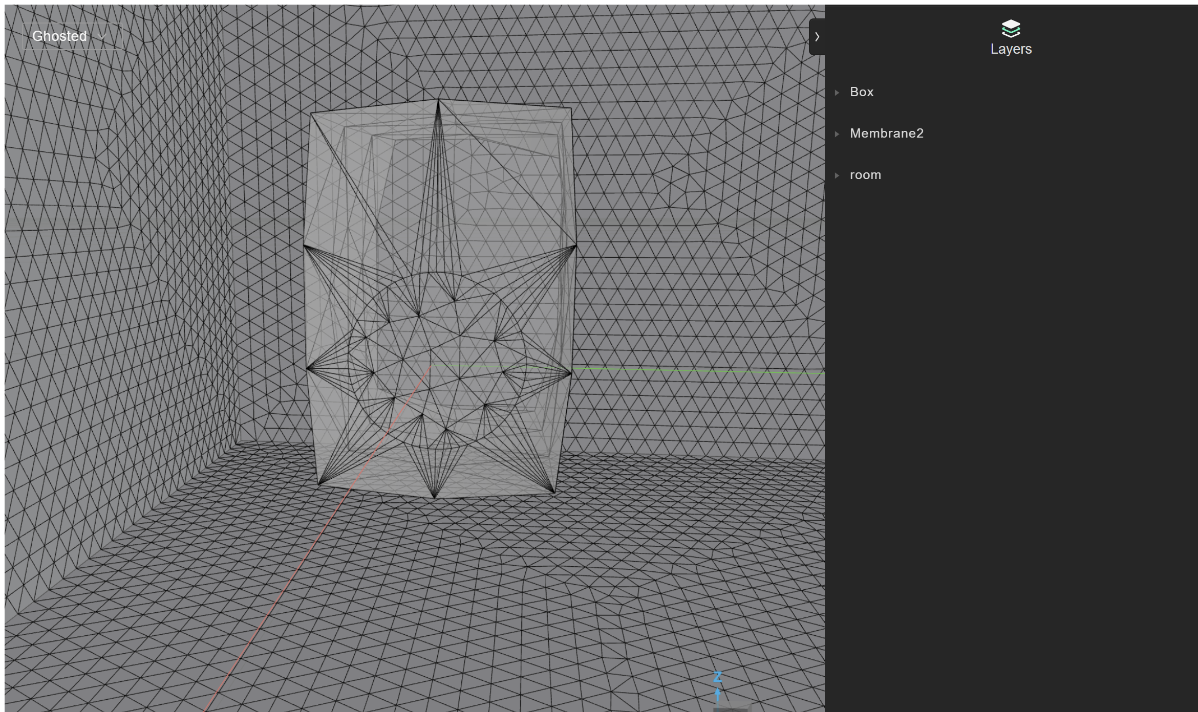
The picture below shows a room hosting a speaker with a circular membrane imported as a model with separate layers in the Treble SDK.

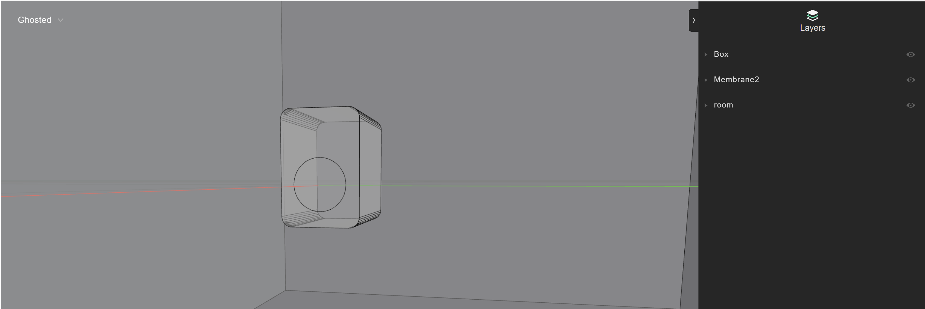
The example code below shows the how to use a global simplification parameter, called simplification_threshold. It refers to lengths in meters and it helps simplifying everything that falls below this threshold. It needs to be used with caution since it can make objects disappear. For example, the speaker above (24cm by 22cm) will disappear with a threshold of 0.3 m, because its dimensions are smaller than this size.

room_model = project.add_model(
        "speakerRoom_1",
        'rhino/SpeakerRoom.3dm',
        geometry_checker_settings=treble.GeometryCheckerSettings(simplification_threshold=0.01),
    )
room_model.wait_for_model_processing()
room_model.plot()

If we apply this parameter when importing a model, we will obtain a geometry without details smaller than the simplification threshold. Below the example geometry with 1cm simplification. We observe how it loses details at the corners.

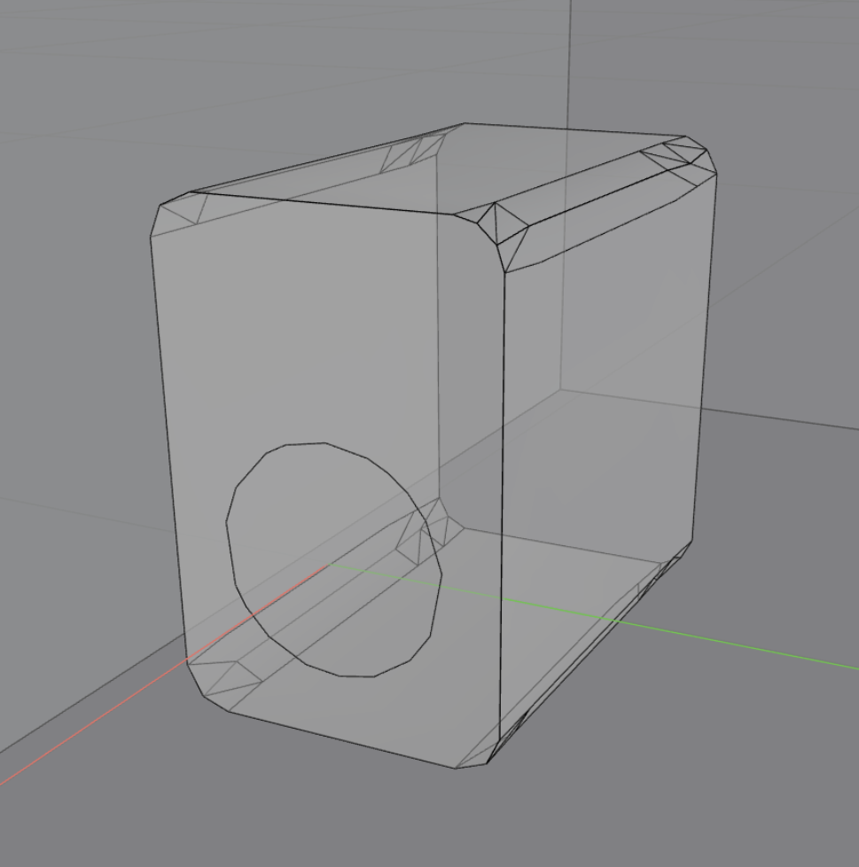
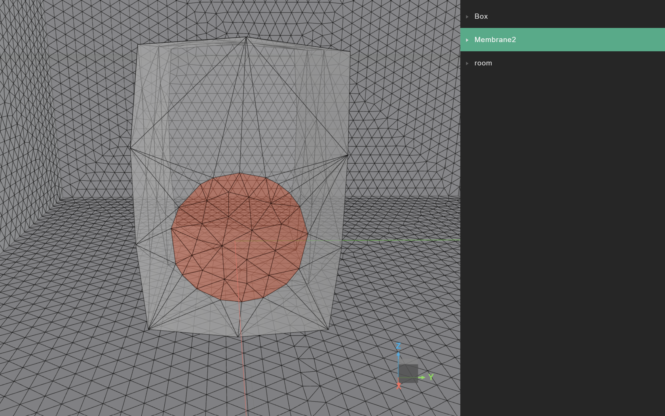
If we proceed setting up a simulation, we will have the simplified model as an input for the volumetric meshing.

As we can observe in this picture, the speaker is lacking detail in correspondence of the rounded edge of the Membrane layer. This has become a diamond. In order to avoid these problems, Treble has introduced a tool to control the mesh sizing with more detail based on the layer, as explained in the next section.

Local sizing

We are left with a simplied speaker that has no detail for the rounded part where the source should be placed. We can amend to this problem by importing the class called LocalMeshSizing and applying these options to the simulation definition, as exemplified below.

from treble_tsdk.core.model_obj import LocalMeshSizing


local_sizing = []

local_sizing.append(
    LocalMeshSizing(
        layer_name="Membrane2",
        mesh_sizing_m=0.01,
        keep_exterior_edges=False, 
    )
)

sim_def = treble.SimulationDefinition(
        name="Test Speaker Room sizing_1cm Edges False ", # unique name of the simulation
        simulation_type=treble.SimulationType.dg, # the type of simulation
        model=room_model, # a room created in an earlier step
        crossover_frequency=3000, # upper limit for DG solver
        energy_decay_threshold=35, # cut off the simulation when the energy decay curve reaches -35 dB
        receiver_list=receiver_list, # two previously defined receivers
        source_list=[source_omni], # one previously defined source
        material_assignment=material_assignment, # the previously defined material assignment list
        local_mesh_sizing=local_sizing
)

sim = project.add_simulation(sim_def)
sim.get_mesh_info().plot()

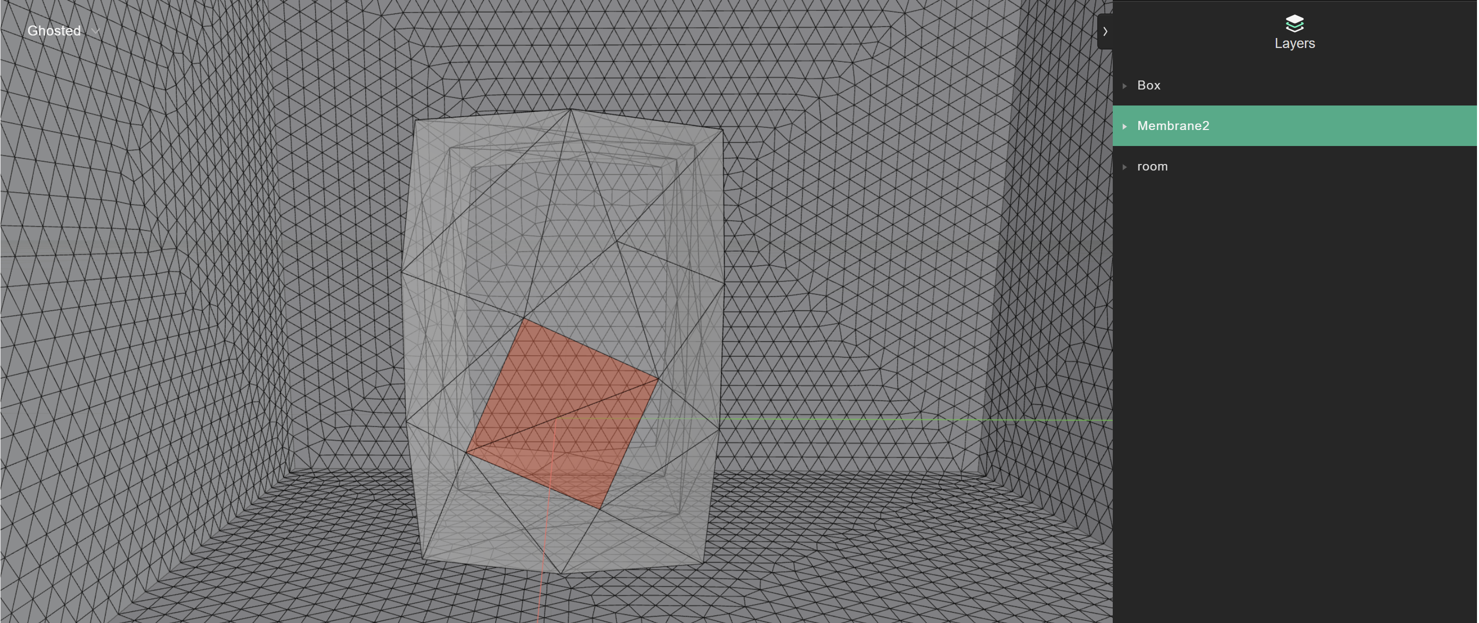
The result from mesh inspection will look as below.

If we want to preserve the rounded shape of the membrane we might just change keep_exterior_edges =True

In the example below, the local sizing for the membrane has been increased to 3 cm, but the edges of the circles are kept. The mesh quality decreases notably since a large number of segments are left on the membrane contour. This will happen if we don't use the previously simplified model that had already a threshold of 1 cm instead of the default of 1 mm.

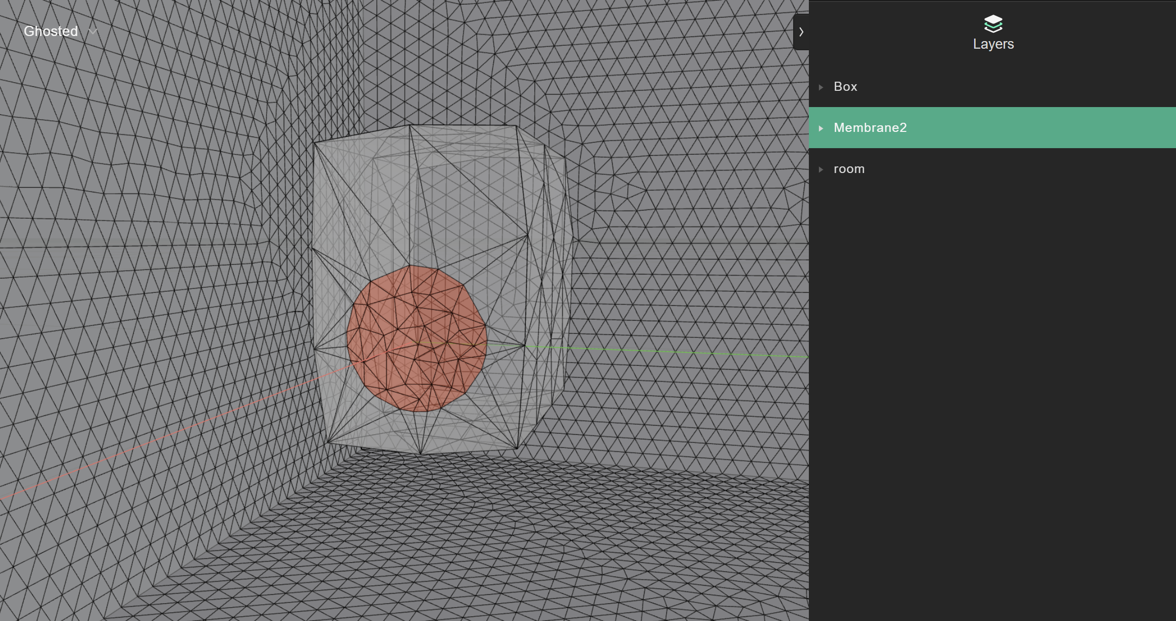
The picture below shows the effect of applying the local sizing of 3cm on the speaker membrane of a speaker previously simplified at the import with a threshold of 1 cm. The mesh efficiency goes from 8% to 24%.

Finally, if we want to transform our membrane in a boundary velocity layer, we can do so by creating a new source using our membrane layer. Local sizing can be specified independently for each layer. In our case the membrane layer is called Membrane2 and it is centered on the origin. When the source_position is not specified it will be created at the center of the layer.

source_boundary = treble.Source.make_boundary_velocity_layer("source_label_membrane","Membrane2", source_position=treble.Point3d(0,0,0) )

Microphone placement on complex object in simulated DRTF

Guidelines

This example illustrates the adoption of a complex geometry to be used for device import. In general, the following rules apply:

• The device should face X axis and be centered on this axis as close as possible to the origin.

• Device microphones should be centered as much as possible.

• Device microphones should be placed on flat surfaces.

The device should be oriented on the X axis so that when it is rotated on the azimuthal plane the correspondences are kept with the rotation in degrees. Positive rotations are calculated counterclockwise from the X axis.

To ensure accurate wavefield resolution, the device must be centered at the origin (or as close as possible) to remain within the required spherical radius. You can read more about how you can analyze your simulated device here.

The microphones and the model should be centered because the tools that creates the elements on which the microphones are placed works optimally when these are centered around the X axis or symmetrical to it.

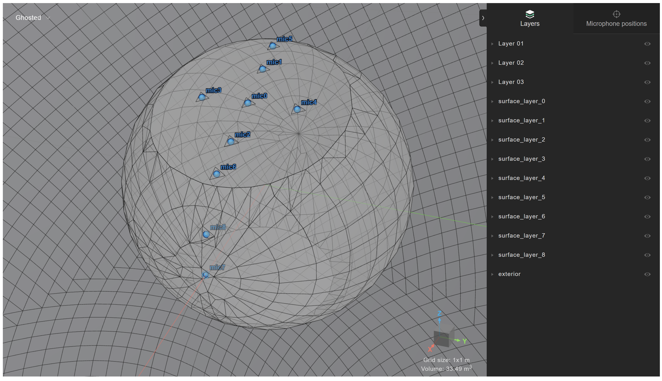
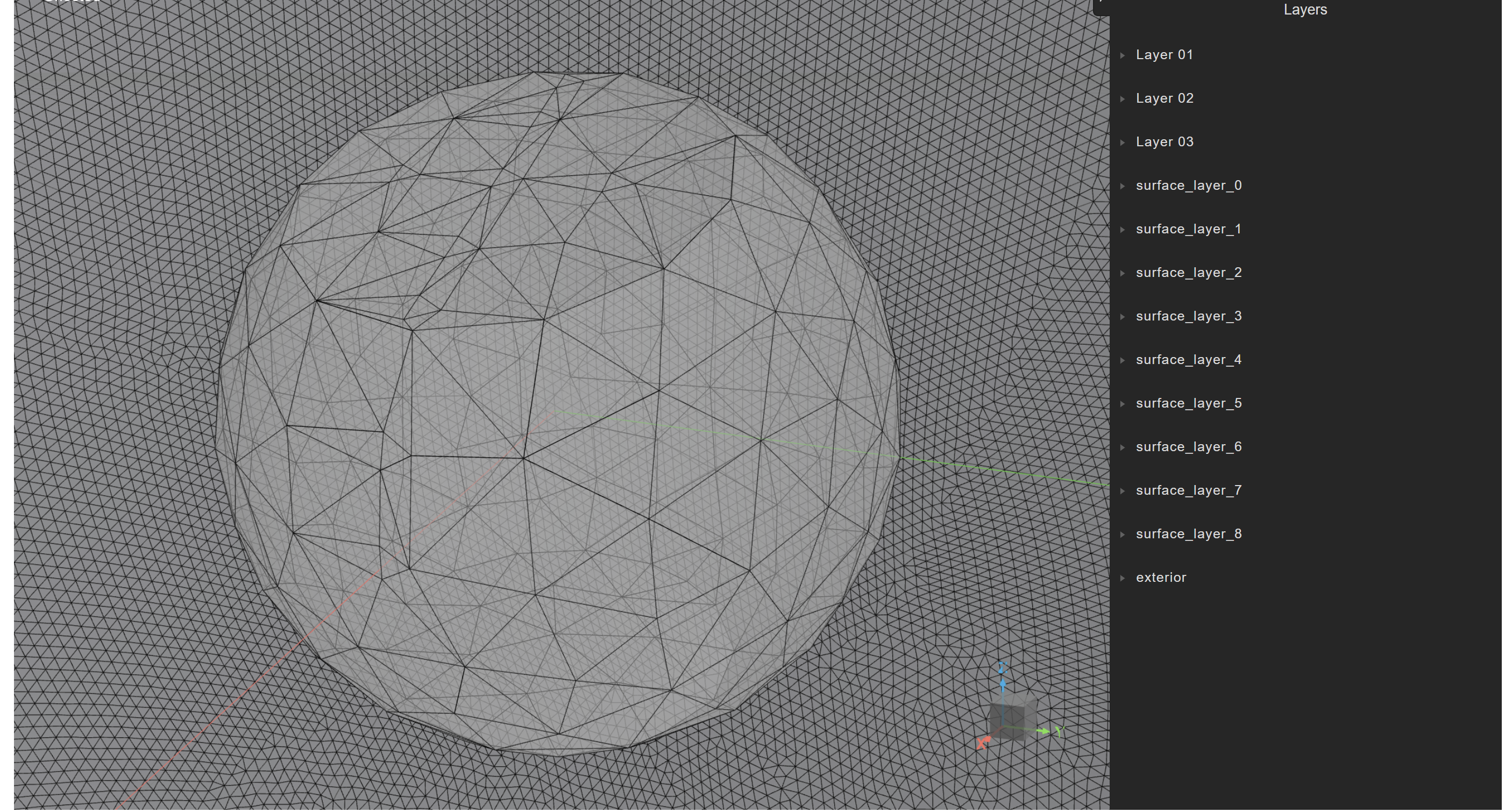
Place microphones directly on a flat surface to avoid generating unwanted geometric artifacts. If placed on a rounded surface, the software automatically creates a small flat area that will protrude slightly.

In the picture below we see a series of microphone placements, both on the flat part of the sphere and the rounded part. The placement of microphones generates small elements, that affects the mesh quality. DRTF simulations are run with very short IR lengths, so here it is generally acceptable to have a suboptimal mesh quality as the run time is short.

Manipulating different levels of detail

In some cases we want to keep high detail in some parts of the device and approximated the rest of its body.

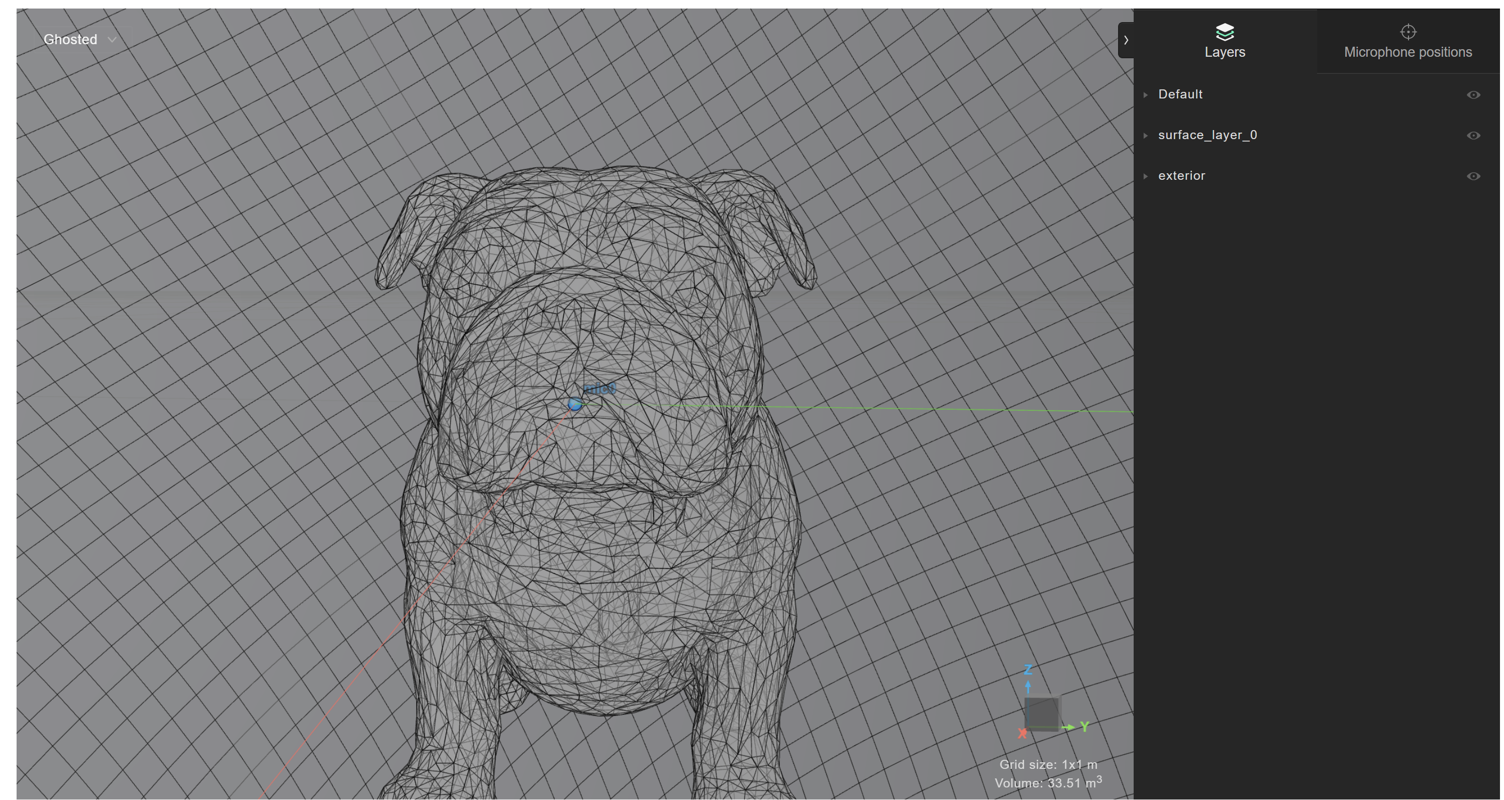
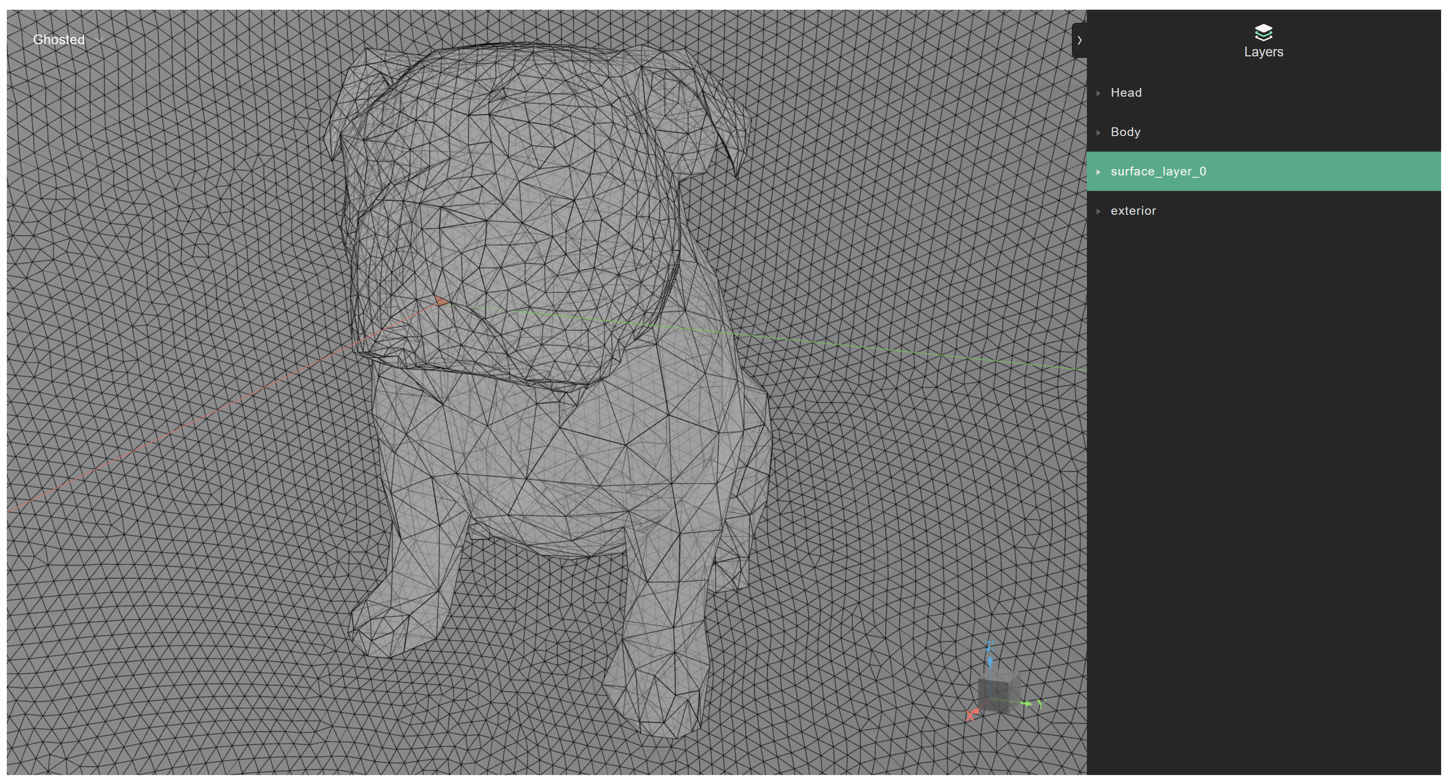
We took as an example a very complex model of a dog and considered whether we could simulate it as a potential device to project sound.

The model was scaled down to fit in a 50 cm radius and simplified down to 10.000 polygons.

It was moved so that the microphone placement would fit exactly on the origin coordinate (0.00, 0.00, 0.00).

We first observe the effect of leaving the default 1mm simplification threshold. The device import was set up as per the code below.

device_name = "dog_speaker"  # Name of the device

device_model_path = "rhino/DogModel.3dm"  # Path to device model
device_microphone_placements = [
     treble.Point3d(0.00,0.00,0.00)

]  # Microphone coordinates of the device
frequency = 6000  # Cutoff frequency
ambisonics_order = 32  # Ambisonics order
n_receivers = round(
    1.5 * (ambisonics_order) ** 2
)  # Number of receivers (spherical array)
receiver_sphere_radius_in_m = (
    1  # Radius of the sphere of receivers for freefield simulation
)
sphere_geometry_radius = (
    2  # Size of the spherical domain for freefield simulation in meters
)
freefield_model_name = "ff_dog_50cm_complex"  # Freefield model name
freefield_simulation_name = (
    "freefield_simulation_dog_50cm_complex"  # Freefield simulation name
)
element_size = 8e-3  # Max. element size for boundary velocity element (device mic)
element_area = (
    np.sqrt(3) / 4
) * element_size**2  # Max. element area estimation based on element size

from treble_tsdk.client.api_models import GeometryCheckerSettingsDto

ff_settings = treble.free_field.FreeFieldModelSettings(frequency=6000, receiver_sphere_radius_in_m=1)

mics = treble.free_field.DeviceMicrophonePlacements(  # Locations and size of the device mic (boundary vel. source)
    list_of_points=device_microphone_placements,     
    injected_triangle_edge_length = 8e-3
)

ff_m = treble.free_field.add_free_field_model(  # Creates the freefield model
    project=project,
    name=freefield_model_name,
    geometry=device_model_path,
    sphere_geometry_radius=sphere_geometry_radius,
    device_microphone_placements=mics,
    freefield_model_additional_settings=ff_settings,
    geometry_checker_settings=GeometryCheckerSettingsDto(
        simplificationThreshold=0.001
    ),
)

from treble_tsdk.core.model_obj import LocalMeshSizing
from treble_tsdk.core.simulation import MesherSettings

local_sizing = []


local_sizing.append(
    LocalMeshSizing(
        layer_name="surface_layer_0",
        mesh_sizing_m=element_size,
        keep_exterior_edges=False,  # Has to be false to have a quality mesh
    )
)

ff_sim_settings = treble.free_field.FreeFieldSimulationSettings(
    number_of_receivers= n_receivers
)
sim_def = treble.free_field.FreeFieldSimulationDefinition(  # Creates the simulation definition
    name=freefield_simulation_name,
    free_field_model=ff_m,
    frequency=frequency,
    receiver_sphere_radius=1,
    source_input="surface_layer_0",
    simulation_purpose=treble.free_field.FreeFieldSimulationPurpose.device,
    free_field_simulation_settings=ff_sim_settings,
    mesher_settings=MesherSettings(simplify_mesh=True),
    local_mesh_sizing=local_sizing,
)
sim_def.plot()

ff_sim = project.add_simulation(
    sim_def
)  # Adds the simulation definition to the project

The local sizing here is addressed by two parameters: injected_triangle_edge_length = 8e-3 and element_size.

The original model looks like this before volumetric meshing.

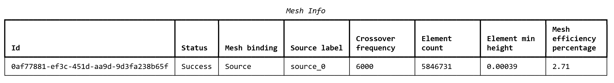
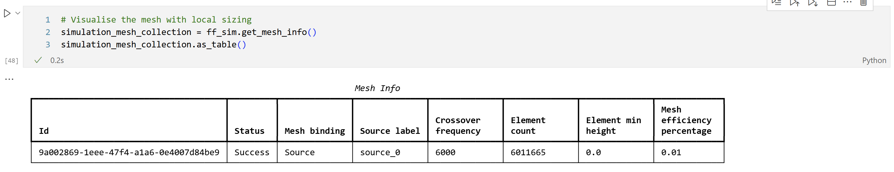
The mesh efficiency is the following without any local sizing beside the microphones, i.e. the injected triangle.

# Visualise the mesh with local sizing
simulation_mesh_collection = ff_sim.get_mesh_info()
simulation_mesh_collection.as_table()

We then apply 1 cm simplification threshold, obtaining this simplified model.

Then we observe the resulting mesh.

source_mesh = simulation_mesh_collection.source_mesh_infos_by_label["source_0"]
source_mesh.plot()

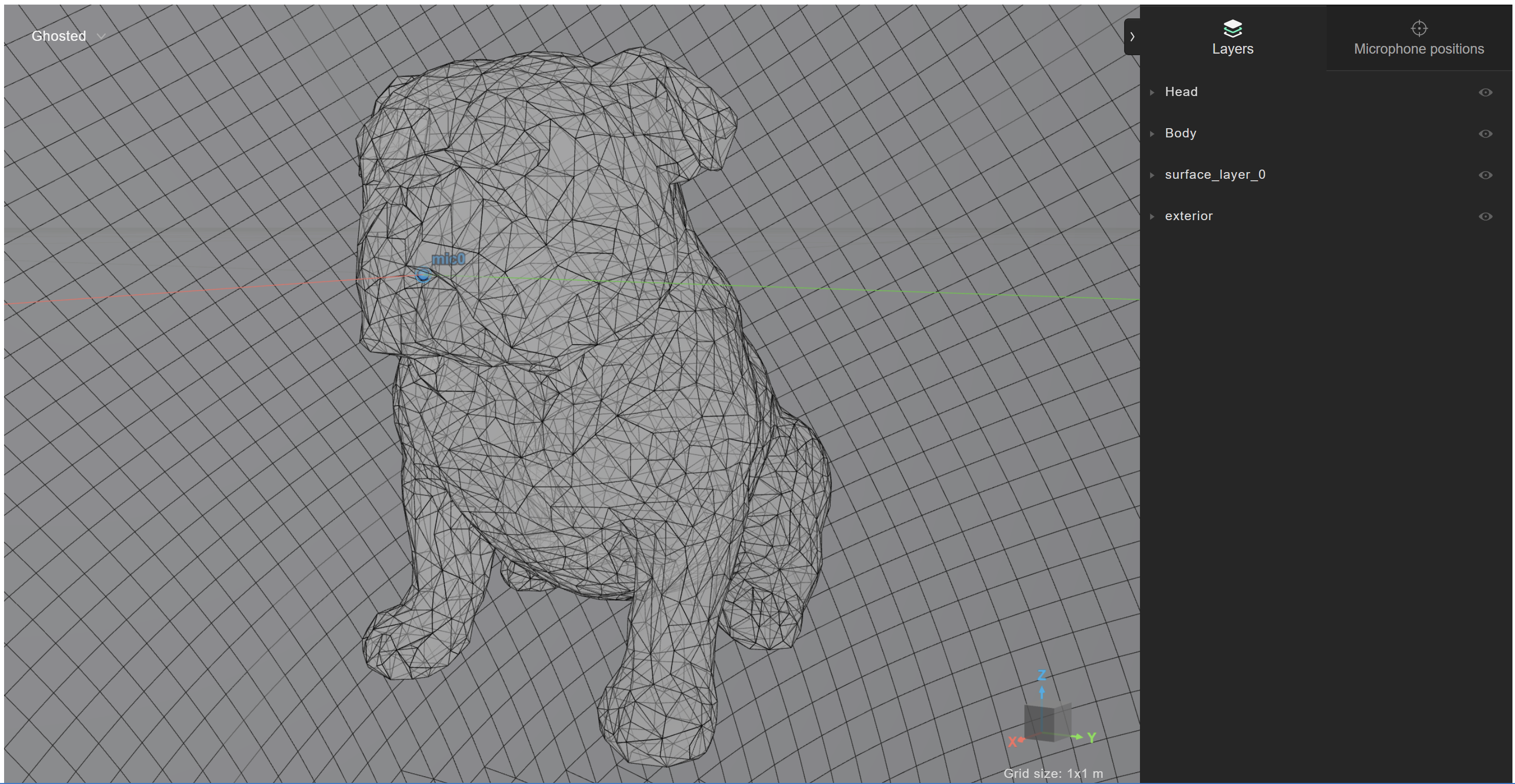
We now want to split the model in two layers, one for the head, one for the body.

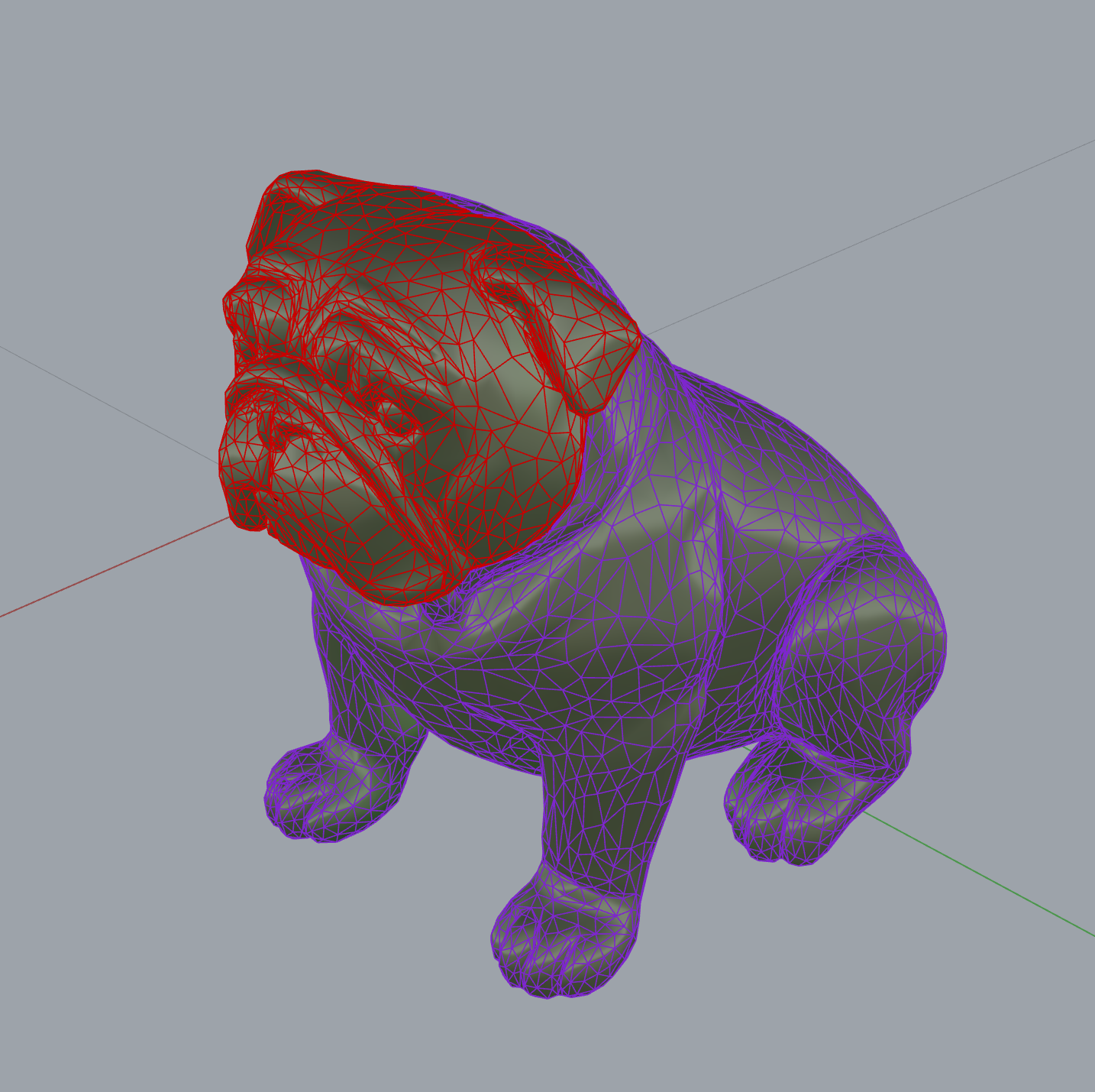
We add another layer sizing and update the simulation definition. Next, we add it to the project.

local_sizing.append(
    LocalMeshSizing(
        layer_name="Head",
        mesh_sizing_m=0.01,
        keep_exterior_edges=False,  # When false mesh might be more efficient
    )
)

In this case, using local sizing to 1cm to preserve features on the face of the model reduces the mesh quality to 0.01%, with a lot of very small elements will not be taken into consideration given the transition frequency of 6000 Hz.

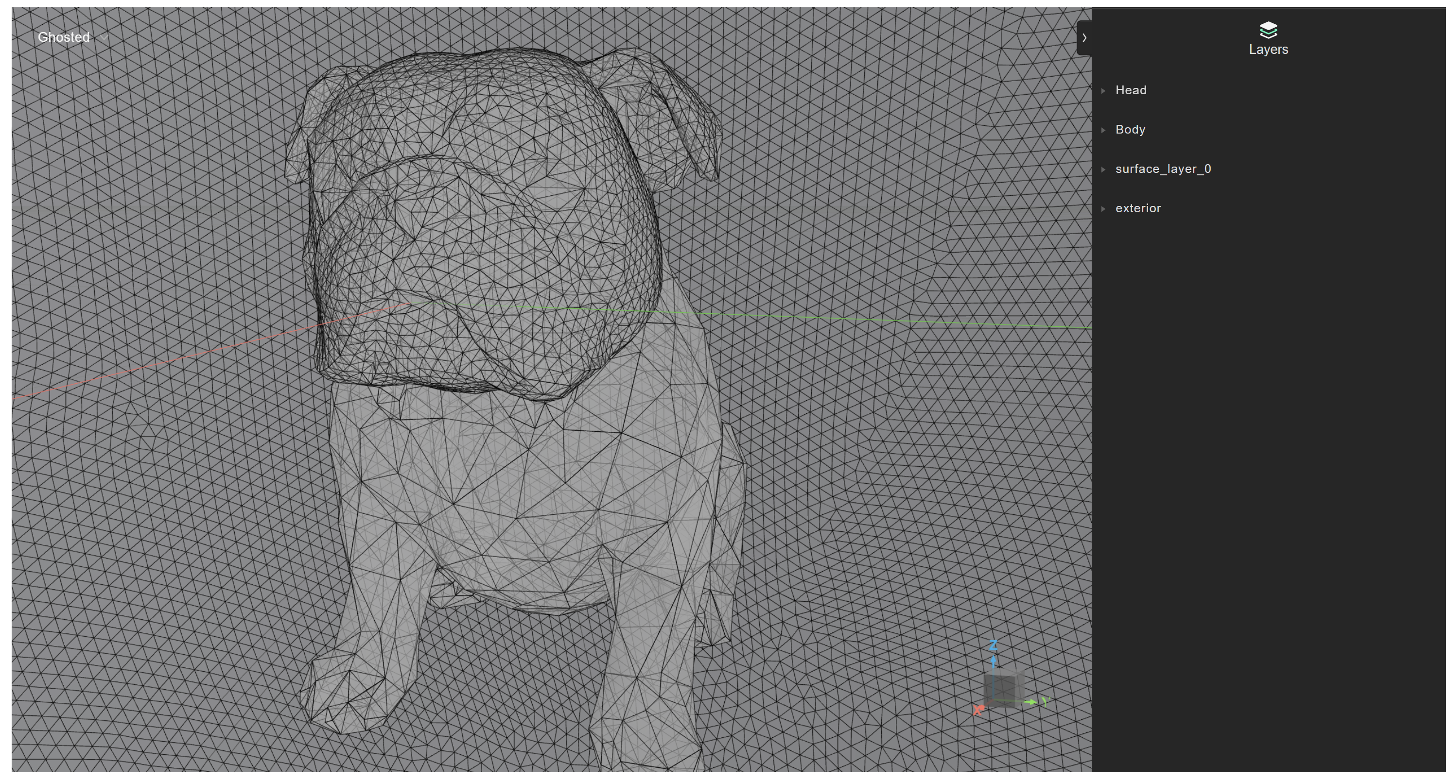
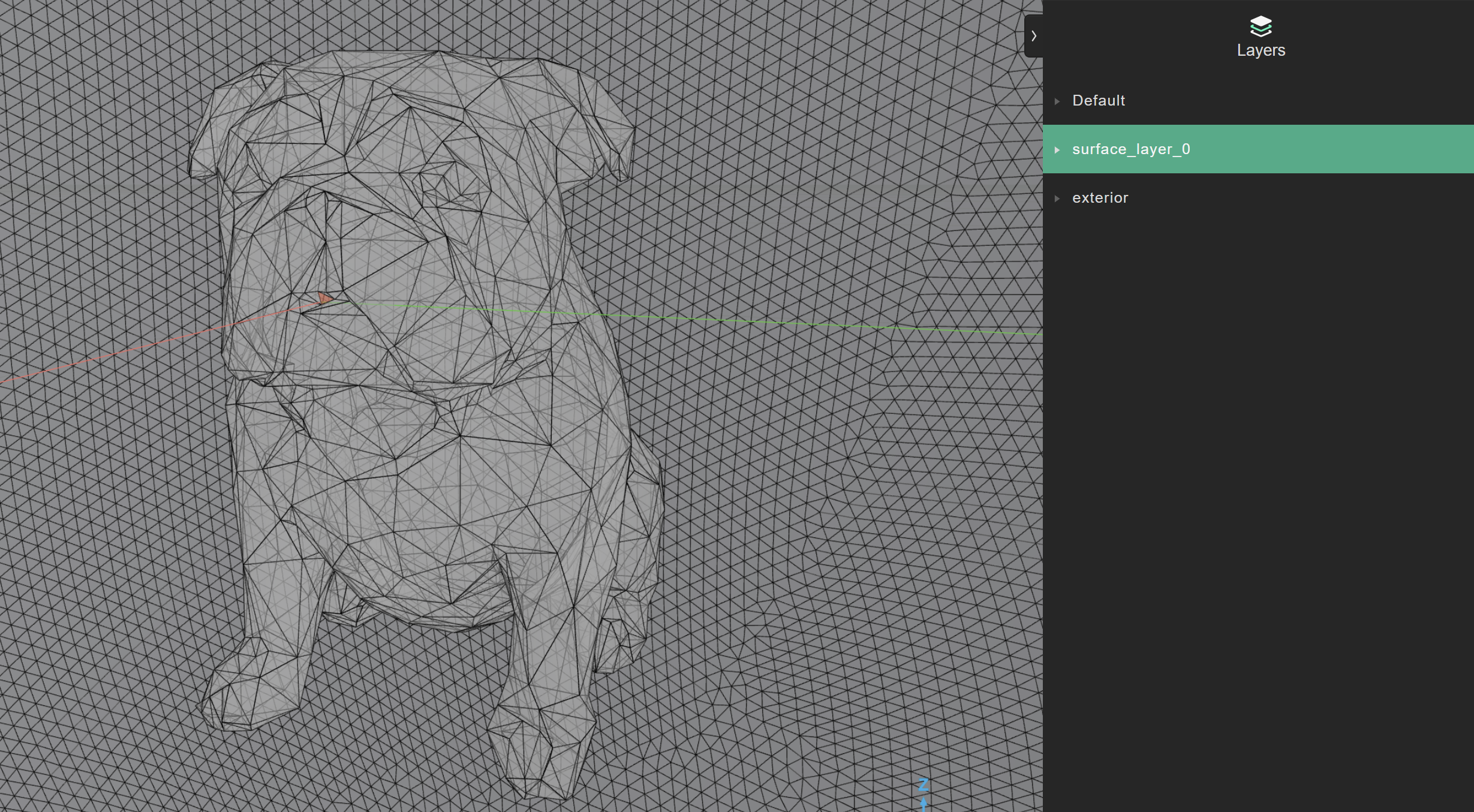
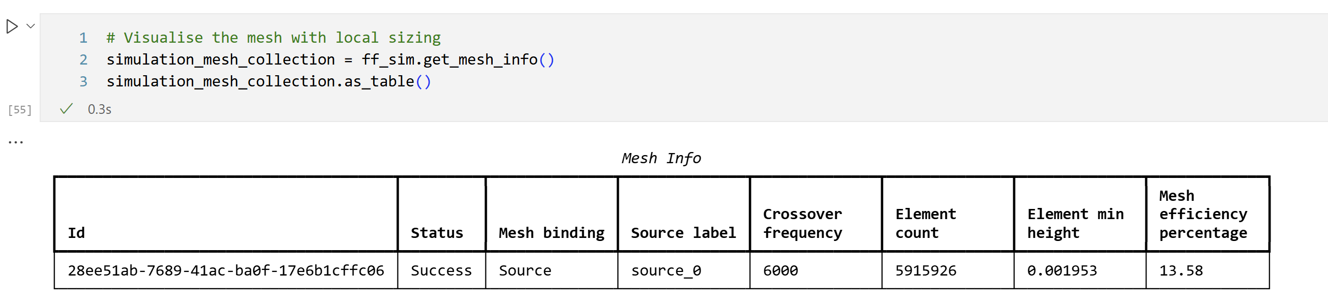
Since the original mesh had already been simplified, we test the effect of removing the simplification from the input geometry, and leaving only the local sizing to operate on the head layer.

The sizing is 1cm on the face, while the rest of the body is automatically simplified by the meshing optimisation process.

In this case, the mesh efficiency is increased to 13%, which is a good step forward. It would be ideal to simplify further the rest of the body.

Simplification off

Below an example of switching off the simplification of small edges by setting the parameter simulation_definition.mesher_settings.simplify_mesh to False.

from treble_tsdk.core.simulation import MesherSettings


sim_def = treble.free_field.FreeFieldSimulationDefinition(  # Creates the simulation definition
    name=freefield_simulation_name,
    free_field_model=ff_m,
    frequency=frequency,
    receiver_sphere_radius=1,
    source_input="surface_layer_0",
    simulation_purpose=treble.free_field.FreeFieldSimulationPurpose.device,
    free_field_simulation_settings=ff_sim_settings,
    mesher_settings=MesherSettings(simplify_mesh=False)
)