Measured DRTF

Importing a measured Device Related Transfer Function (DRTF)

DRTFs are a useful tool for placing complex device geometries into the simulated sound field in post-processing using Spatial Room Impulse Responses (SRIR) and very high-order-ambisonics (HOA).

The device rending stage happens after the completion of the simulation. This allows for easily testing multiple device designs as well as multiple orientations, from the same simulation run.

The device geometry can range from a small device placed on a table with multiple microphones to a complex head and torso model with detailed ear pinna and ear coupler resonances at the eardrum microphone.

An alternative to the DRTF approach is to place the device geometry within the room geometry. However, this means that the device and its orientation are fixed, requiring a new simulation for each new device type or orientation.

When importing a measured DRTF it is the user's responsibility to ensure sufficient quality of the DRTF, both during the measurement itself and in the post-processing of the results.

The principle of GIGO (Garbage in, Garbage out) truly applies in this case. All faults in the measured DRTF will be transferred to the rendered results using said DRTF.

In this guideline we will cover the necessary steps to get the best possible results.

Measurements setup

Number of sources

The measurements needs to have a minimum amount of sources placed in a sphere pattern around the device under test (DUT).

To give a frame of reference, encoding a DRTF up to ambisonics order 16 requires about 440 source directions. In this case, the rule 'the more, the merrier' applies It is better to have an overdetermined system than underdetermined.

It is not uncommon for automated measurement systems to have somewhere between 1500-3000 different source locations, depending on the discretization grid of the sphere.

The most common approach is to have evenly discretized spacing of the azimuth and elevation, but other patterns, such as Fibonacci or Lebedev patterns, also work well.

Azimuth and Elevation

The sphere of sources around the device should have a minimum radius of approximately 1 meter. A larger sphere could be beneficial for larger devices, such as head and torso simulators.

Ideally, the whole sphere should be sampled without leaving any "gaps" in the data, including for the directions corresponding to low elevations (i.e., below the horizontal plane). This is not always easy to achieve during measurements without the generation of spurious reflections from the measurement setup, for instance, due to semi-anechoic conditions. The response for the missing directions will be automatically inferred from a regularization procedure. This typically results in localized shadow zones for the missing directions, which can lead to an underestimation of the sound waves coming from beneath the device.

In those cases the lowest negative elevation angle results will be copied over the the missing angles, in order to have a complete sphere result. The consequence is that a small shadow zone will form below the device, resulting in underestimated reflections coming from beneath the device.

Luckily this area has a low density of reflections for devices commonly placed on tables, and also for humans standing on legs or sitting in chairs.

At Treble, we have tested and verified DRTF datasets measured down to -60° elevations with good results.

The placement of the device should be in the middle of the sphere with the average center point of the microphones on the device as the origin. As an example, the HRTF of a head and torso should have the center of head, between the ears, as the origin (0,0,0) as illustrated below.

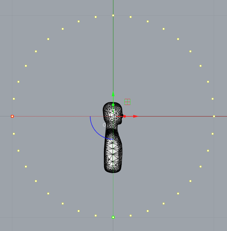
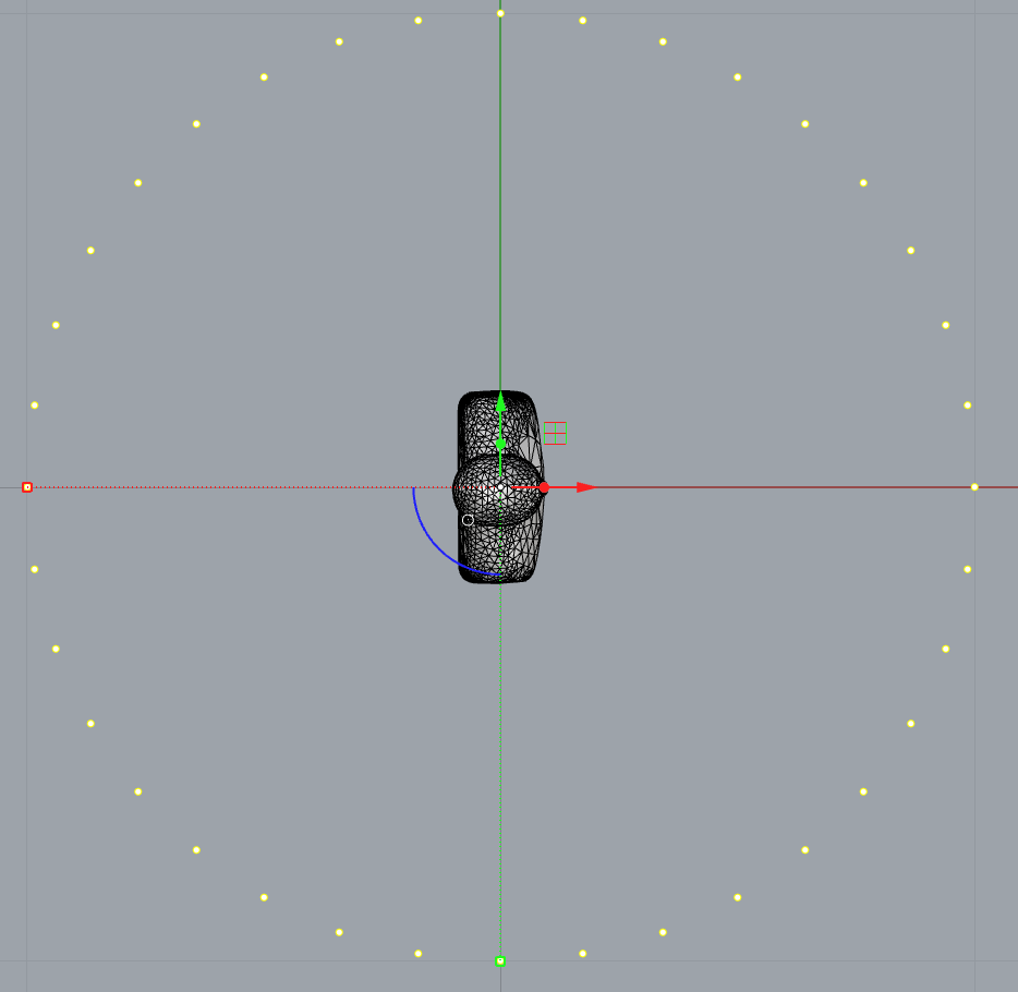
For devices with all the microphones placed on top of the device, the origin should then be on top of the device.

Post-Processing

When measuring a DRTF with an external loudspeaker it is recommended to measure the free field response of said loudspeaker (or loudspeakers if working with a multi-speaker setup). The free field response should then we removed from the DRTF measurements, unless it is desired to have the effect of the external loudspeaker included in the DRTF data. The loudspeaker response can be removed with a simple FFT division in the frequency domain. This operation must be regularized to avoid division by small numbers (and thus the amplification of noise). This can be achieved for instance with the following formula, with regularization_parameter set to an appropriate value:

$$\text{fft\_eq} = \frac{\text{fft1} \cdot \text{conj}(\text{fft2})}{|\text{fft2}|^2 + \text{regularization\_parameter}}$$

where $\text{fft\_eq}$$ is the final free-field-corrected results, $\text{fft1}$ is the FFT of the measured DRTF and $\text{fft2}$ is the fft of the free-field loudspeaker measurement.

The following plot illustrates the presence of a notch in the loudspeaker free-field measurement.

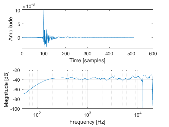
When dividing with this response in the frequency domain the resulting IR is shown on the following plot, with and without regularization of the FFT division.

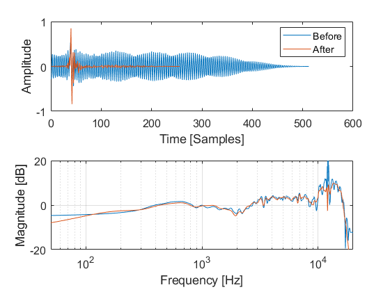
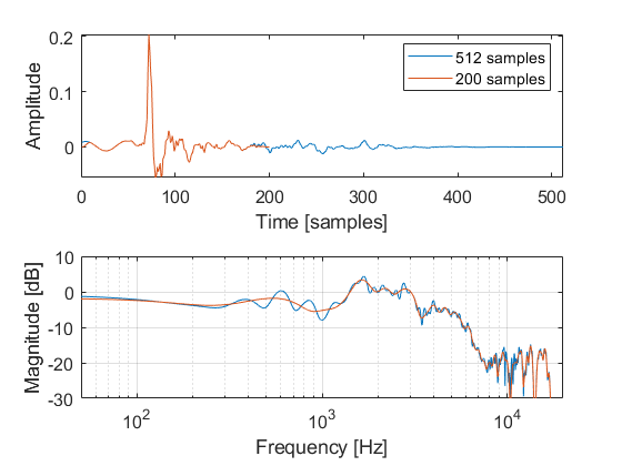
Finally, we recommend an aggressive time-windowing of the device data to taper out any parasitic reflections from the measurement setup, which may degrade the accuracy of the ambisonics representation of the device. Most of the information contained in the DRTF (or technically, the DRIR) are typically captured in the first 3-5 ms, or 150-250 samples assuming a 48 kHz sampling frequency.

The following plot shows how the shorter time window effectively smooths the DRTF response in the frequency domain.

Importing Measured Data

To import a DRTF, we need the azimuth and elevation angles in degrees and an impulse response or transfer function for each angle for all the microphones on the device.

To illustrate the import functionally, we use in the following the HRTF dataset of a KEMAR mannequin measured and provided by the Reality Labs research group
https://facebookresearch.github.io/SS2_HRTF/

We recommend to multiply the response with the sampling frequency, to avoid any loss of energy later on when the results get downsampled to 32kHz.

We also recommend to have a short window to avoid reflections as is explained above. In this first example we include both of these operations and do the import step by step.

In the second example below we take the short-cut and import directly from the sofa file.

import numpy as np
import h5py

# Define parameters
window_length_samples = 200  # in samples
fade_length = 50  # in samples
# Create a Hann window
hanning_window = np.hanning(fade_length * 2)
# Extract the fade-out portion
fade_out = hanning_window[fade_length:]
# Create the final window
final_window = np.ones(window_length_samples)
final_window[-fade_length:] *= fade_out

# We know the microphone names in the file and loop through them
microphone_names = ["left", "right"]
device_microphones = []
with h5py.File("KEMAR051123_1_processed.sofa", "r") as f:
    
    # All the microphones share the same source locations
    source_positions = treble.DeviceSourceLocations(
        azimuth_deg = f["SourcePosition"][:,0],
        elevation_deg = f["SourcePosition"][:,1],
    )

    for n in range(np.size(microphone_names)):
        
        # Here we read in the impulse responses for each microphone and
        # append a DeviceMicrophone object to the list of microphones

        # load IR
        ir_temp = f["Data.IR"][:,n,:]
        # Scale with the sampling frequency
        ir_tempfs = ir_temp * f["Data.SamplingRate"][:]
        # add window
        ir_tempfswin = ir_tempfs[:,0:window_length_samples] * final_window

        impulse_response = treble.DeviceImpulseResponses(
        impulse_responses = ir_tempfswin,
        sampling_rate = f["Data.SamplingRate"][:],
        )
        device_microphones.append(
            treble.DeviceMicrophone(
                source_locations = source_positions,
                recordings = impulse_response,
                max_ambisonics_order = 16,
            )
        )

Give the device a name and a description

device_definition = treble.DeviceDefinition(
    device_microphones=device_microphones,
    name="KEMAR051123_1",
    description="KEMAR from Meta database, scaled with fs and windowed",
)

And finally import the device to your library

device = tsdk.device_library.add_device(device_definition=device_definition)

In case you are confident in the quality of your sofa file and just want to get in there fast and easy the next example should do the trick.

This does not include the shorter time window or the scaling by the sampling frequency.

Note that sofa files, even though they are standardized, can vary in data format. This import method was tested with the Reality Labs sofa format

# import sofa file directly
from treble_tsdk.postprocessing.DRTF import create_device_from_sofa_file

device_definition = create_device_from_sofa_file(
                    sofa_filepath = "KEMAR051123_1_processed.sofa",
                    device_name = "KEMAR_sofa",
                    max_ambisonics_order = 32 ,
                    device_description = "KEMAR from sofa file")

device = tsdk.device_library.add_device(device_definition=device_definition)

List all the available devices to make sure your import worked

dd.as_table(tsdk.device_library.get_devices())