Quick start guide
Welcome to this tutorial in which we will guide you through running a simple simulation, obtaining results and setting up an auralization, using the Treble Web App.
1. Navigating the home page overview
After you have activated your Treble account, open Treble by navigating to app.treble.tech on your internet browser of choice. There, you’ll be presented with the home screen. On the home screen you will see all of your recent projects and spaces. An example project is pre-loaded by default, featuring four pre-configured spaces to explore.
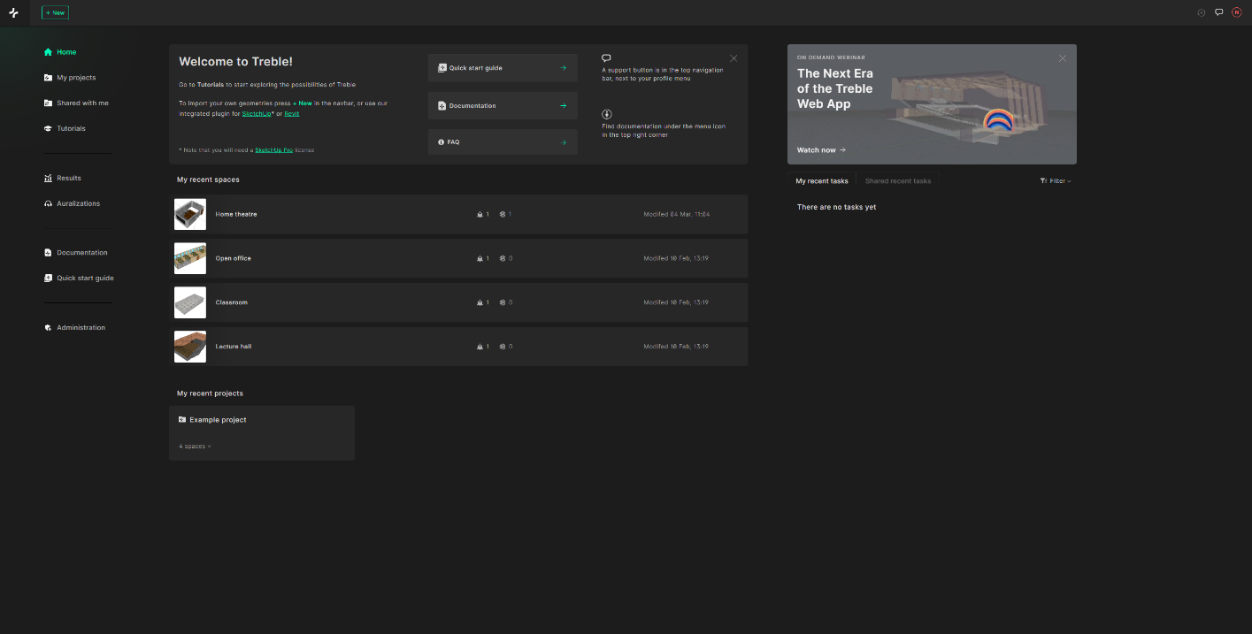
Select the classroom from the list of recent spaces.
2. Creating a simulation
You are now in the Model Editor, where you can create and run simulations.
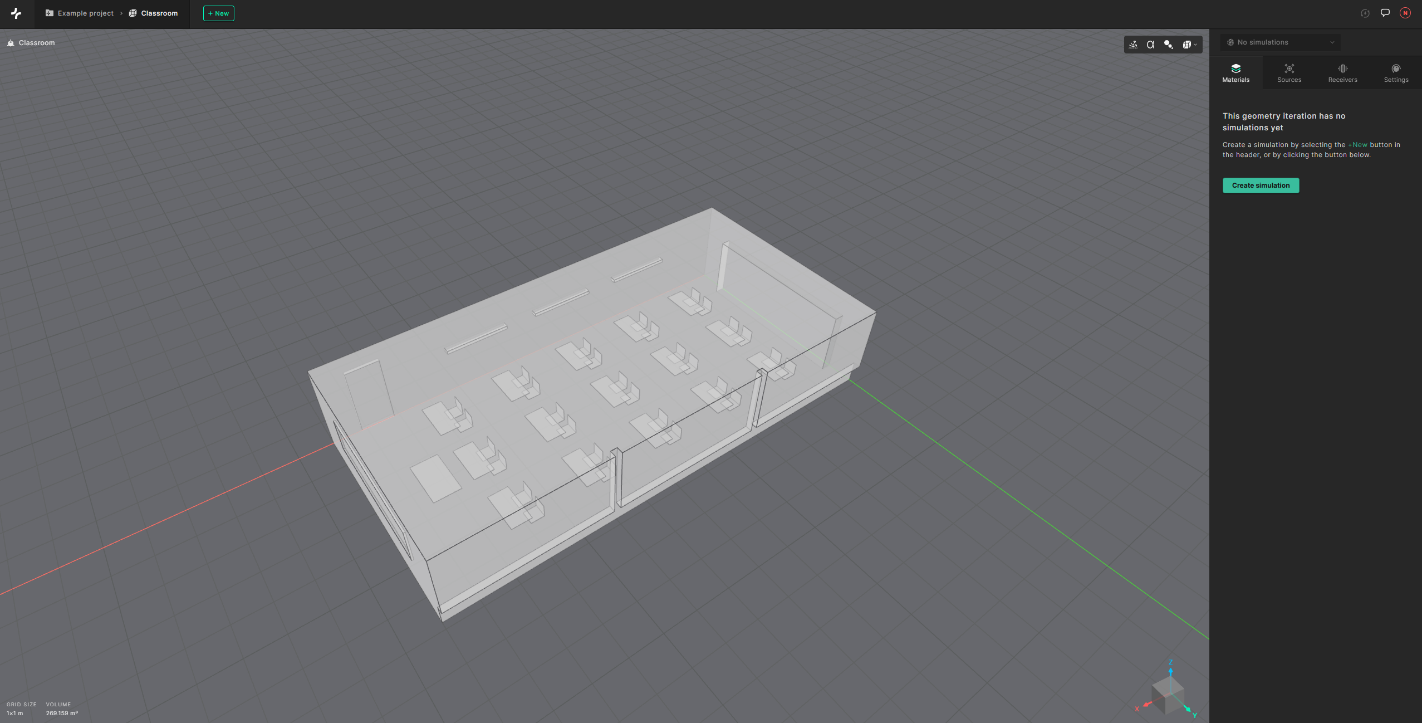
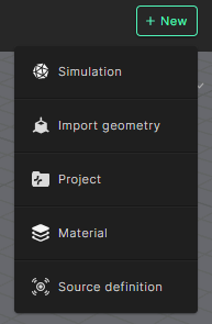
To set up a new simulation you can either select ‘Create simulation’ in the side panel on the right, or click the ‘New’ button, this is visible in the application header. Choose ’Simulation’ from the list that appears.
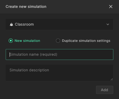
Choose a name for the simulation in the ’Simulation name’ field. You can also add your own description and notes in the ’Simulation description’ field.
3. Material assignment
The first step in creating a simulation is to assign materials and material properties to all surfaces in the model. To assign materials, select the relevant layer or surface in the list of layers on the right.
You can assign materials to multiple surfaces at once by holding down ‘Ctrl’ or ‘Shift’ on your keyboard.
Start by clicking the ’Unassigned’ input for the ’Walls’ layer. The selected surfaces get highlighted in the model and the material library appears.
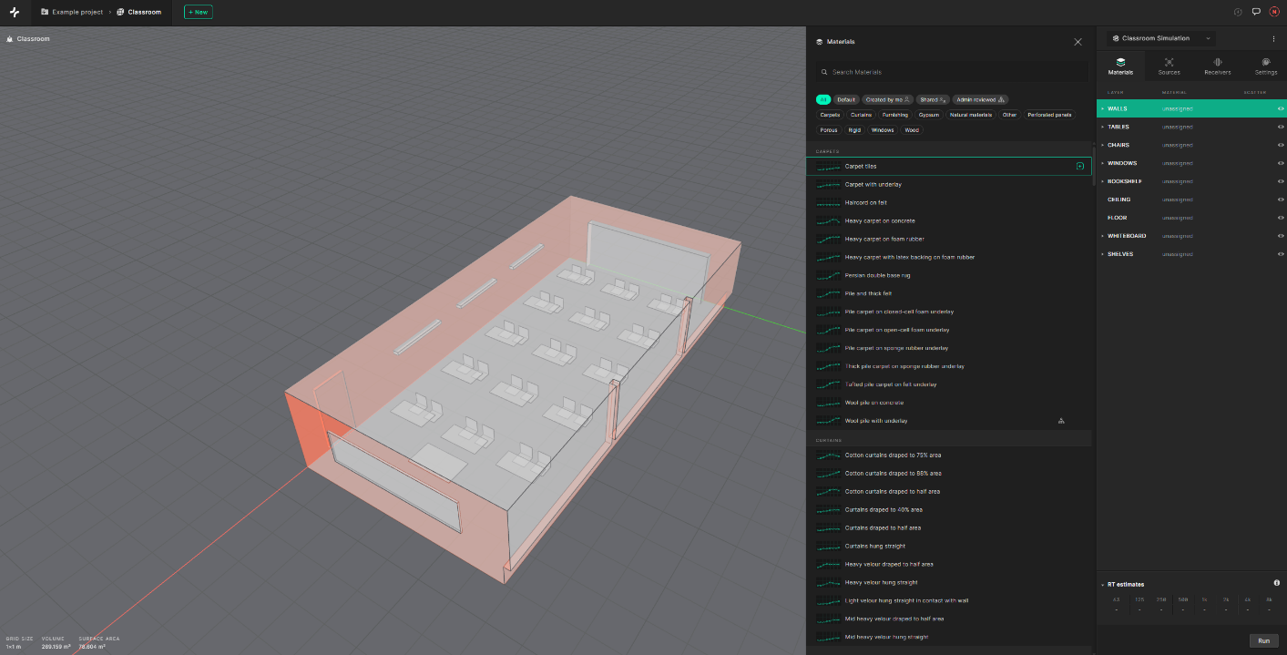
To easily search within the material library, you can use the search bar at the top, or filter materials using the tags.
Firstly, let’s assign a material to the ’Walls’ layer. Select the ’Gypsum’ tag and select the “13 mm Gypsum/Plaster board on frame, 100 mm mineral wool behind” material. You can also use the search bar to find it.
Click on the ’+’ icon to assign the material to the wall.
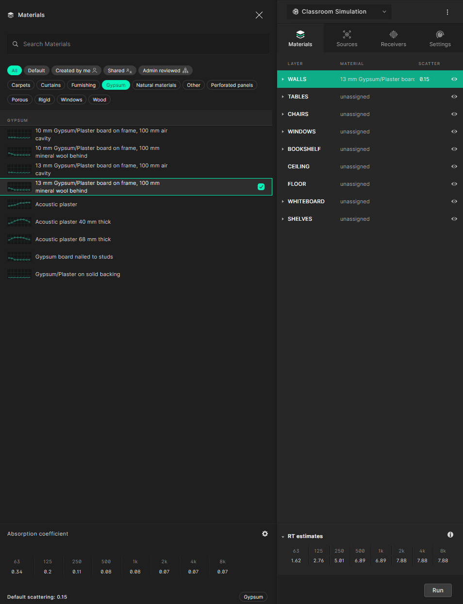
The wall has now been assigned a material. A default scattering coefficient of 0.15 has also been assigned. The default scattering values should cover a broad range of applications but we recommend evaluating and adjusting them on a case-by-case basis as explained in the scattering best practices guide.
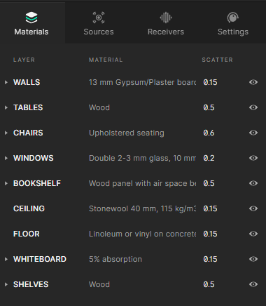
For this tutorial we recommend assigning the following materials on each layer:
- Tables > Wood
- Chairs > Upholstered seating
- Windows > Double 2-3 mm glass, 10 mm air gap
- Bookshelf > Wood panel with air space behind
- Ceiling > Stonewool 40 mm, 115 kg/m3
- Floor > Linoleum or vinyl on concrete
- Whiteboard > 5% absorption
- Shelves > Wood
For the scattering coefficients on this specific model, we recommend the following scatter values:
- Walls > 0.15
- Tables > 0.5
- Chairs > 0.6
- Windows > 0.2
- Bookshelf > 0.5
- Ceiling > 0.15
- Floor > 0.15
- Whiteboard > 0.15
- Shelves > 0.5
After assigning all the materials and their properties, your material setup should look like this:
The ’RT estimates’ tab in the bottom right shows the estimated reverberation time in the room based on Sabine’s equation. The equation assumes a completely diffused sound field and doesn’t account for the location of absorbers or diffusers. It’s therefore mainly meant for reference to help you dial in your simulation setup before you run a more thorough simulation.

4. Setting up sources and receivers
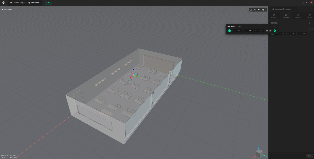
You are now ready to set up the sound sources and receivers in the room. Click on the Sources tab.
To define a new sound source, click on the ’+ Add’ icon next to ’Sources’. An omnidirectional source will be created by default.
You can either position a source by dragging it along the dimensional axis or by defining precise coordinates. Treble also has a range of ways to group, multiply and transform sources and receivers which will be of great use as you get more experience in the platform. For this tutorial, you can place a source at the following coordinates:
- X: 5.5 – Y: 2.5 – Z:1.5
The process of placing a receiver is the same as placing a source.
Navigate to the ’Receivers’ tab and click on the ’+ Add’ icon to the right of ’Point Receivers’ and place a receiver at the following coordinates:
- X: 10 – Y: 5 – Z:1.5
Then click on the “+” icon again and place additional receivers at the following coordinates:
- X: 3 – Y: 1.5 – Z:1.5
- X: 12 – Y: 4 – Z:1.5
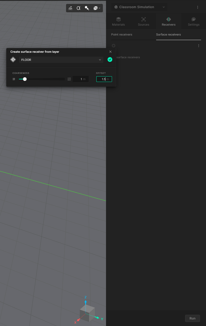
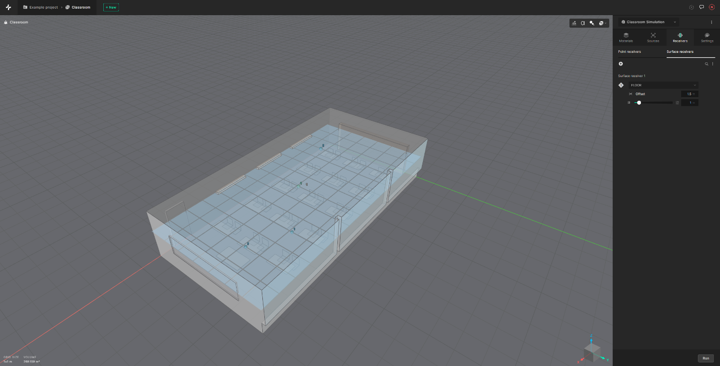
We will now place a surface receiver in the model to get a visual interpretation of the distribution of parameters within a room. To do that select the ’Surface receivers’ tab and click on the “+” icon.
Within the Surface Receivers tab, we will ’Create from layer’ and will then select the ’FLOOR’ layer. This method is called ’offsetting’ which will create a surface receiver from an already existing geometric surface. This can be a quicker way of generating large surface receivers instead of needing to create, size and position one manually (which is also possible).
The coarseness slider enables you to set the dimensions [length and width] of each individual square grid element. For this tutorial, you can leave them unchanged at 1 m. You can also use an offset height of 1.5 m.
If creating a surface receiver from a ’Custom Grid’, to quickly cover a whole surface with a receiver grid, create a surface receiver that extends beyond the boundary of the room. Treble will automatically discard the receivers outside the geometry.
5. Simulation settings
The last step before running a simulation is to set your simulation settings. Click on the Settings tab. Within the settings tab you can select between the following:
- Survey: Quick simulation using only the geometrical solver
- Default: The highly accurate wave solver is used up to an automatically estimated frequency. Above that frequency the geometrical solver is used. This is the recommended setting when starting with Treble and will be used for this tutorial.
- Advanced: Allows the user to customize the transition frequency between the wave solver and the geometrical solver. It also allows for changing the number of rays the geometrical solver sends out, amongst other advanced features.
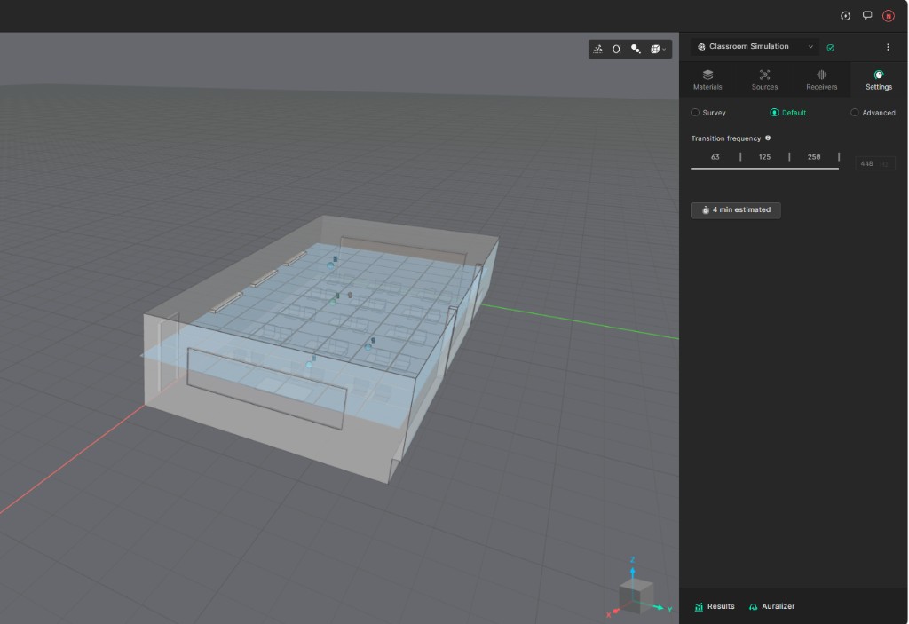
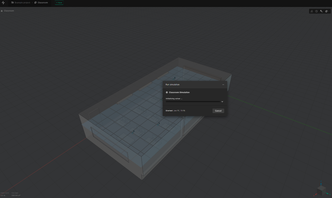
Select Default and click on “Run”. A popup will show information about the key properties of the simulation:
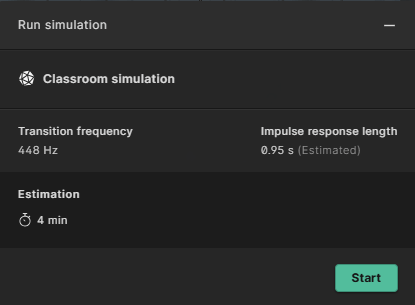
Click ’Start’ when you’re ready to run the simulation.
After starting the simulation, you can safely minimize the “Simulation run” popup window and work within Treble as normal while the calculations take place in the cloud. You can stop a simulation at any point by clicking on “Cancel”.
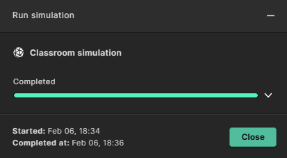
Once the simulation is finished you can press “Close” in the ’Simulation run’ window if you still have it open.
6. Results and analysis
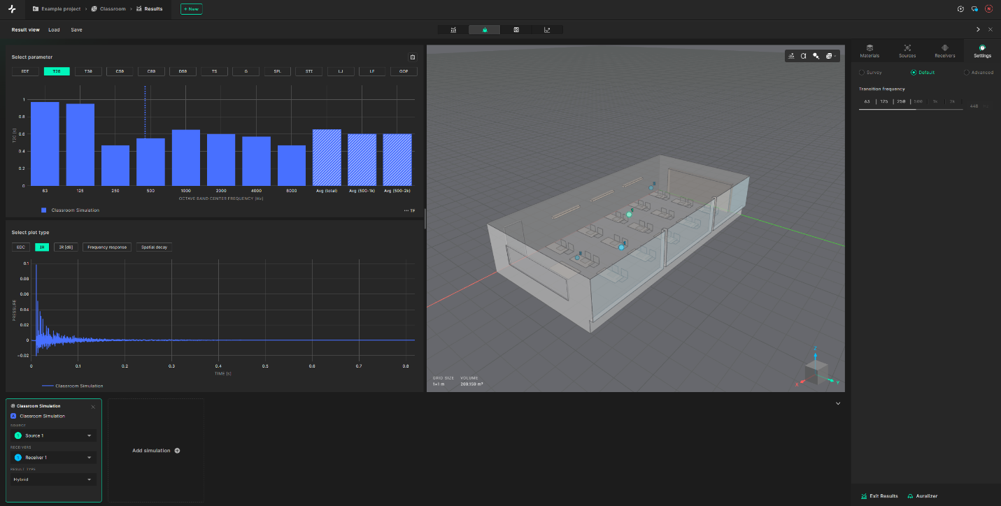
You are now ready to view the results of your simulation. Head to the results view in the bottom right.

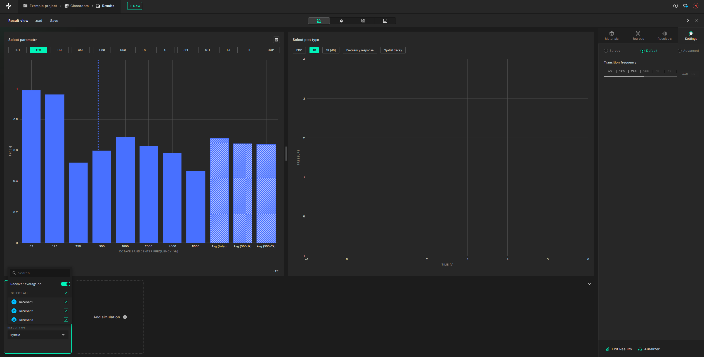
Within this view you can see the results of the different calculation parameters.
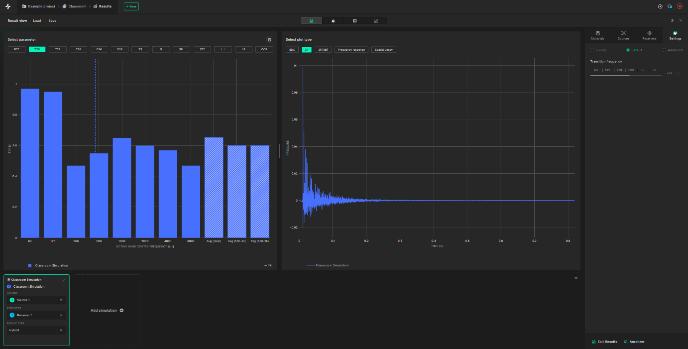
By selecting the ’Report view’ button at the top (highlighted in green below), you can see more plot results displayed in a larger format.
We encourage you to try out all our different features within the results view. The bar graphs on the left show all the calculated acoustic parameters that Treble offers.
The plots on the right show the simulated impulse response, energy decay curve and frequency response. You can see the calculation results averaged over multiple receivers or for summed sources. To average across receivers, select the receiver tab at the bottom, turn the multiselect toggle on and check the ’select all checkbox’. For this simulation we only have a single source so source summing is not enabled.
You can also compare different simulations by adding a new simulation that has been run to the results graph using the plus icon at the bottom.
You can see acoustical parameters across the surface receiver view by selecting ’surface receivers view’ at the top. When a wave simulation has been run, you will also be able to use the more advanced view types ’Forced Modal Analysis’ and ’Wavefield Animation’.
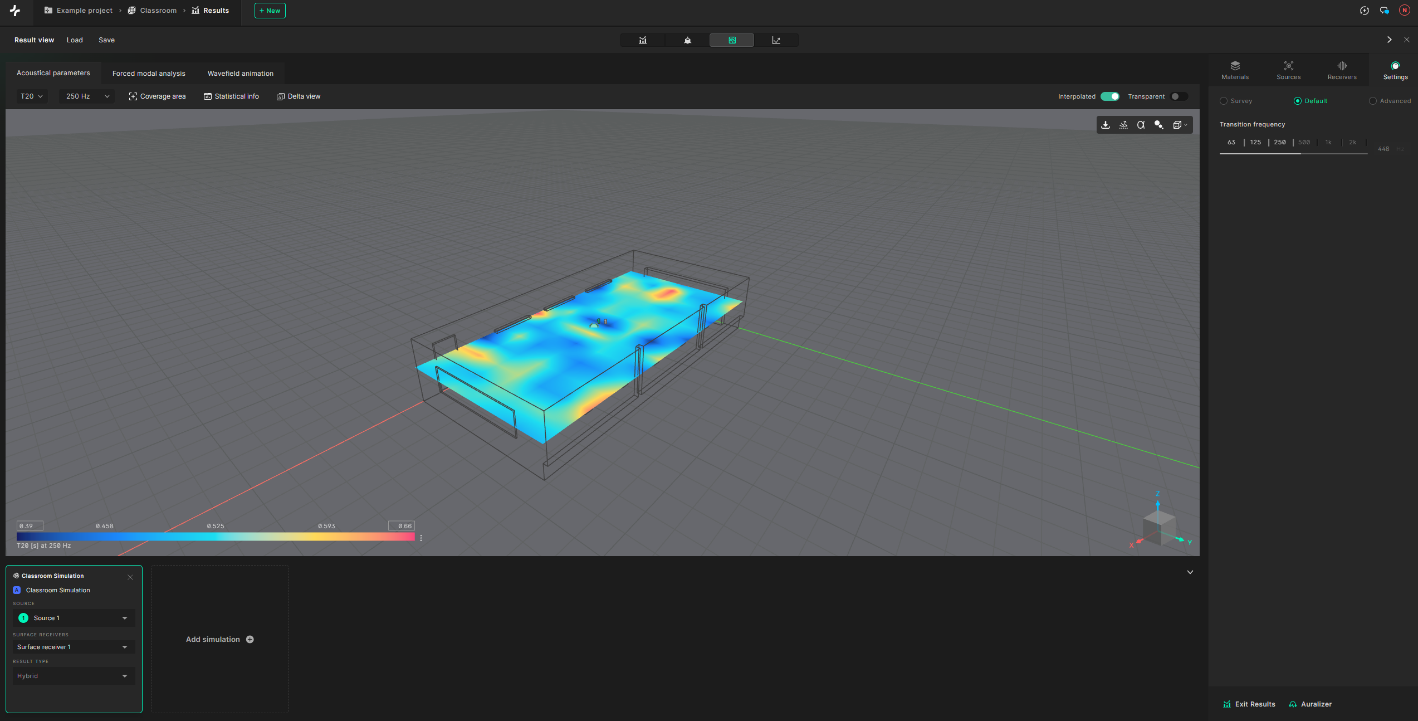
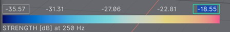
You can edit the min. and max. values of the axis to directly compare the surface receiver results of different simulations.
7. Auralizer
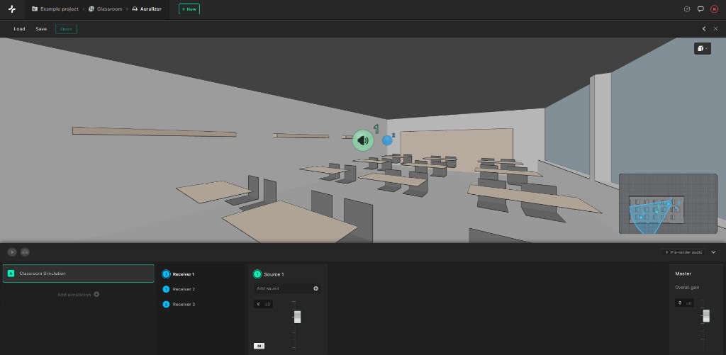
The final step of this tutorial is to listen to your results in the auralizer. Click on “Auralizer” in the bottom right.

Within the auralizer view, you can select individual receivers to listen to the acoustics of the room at their respective various locations.
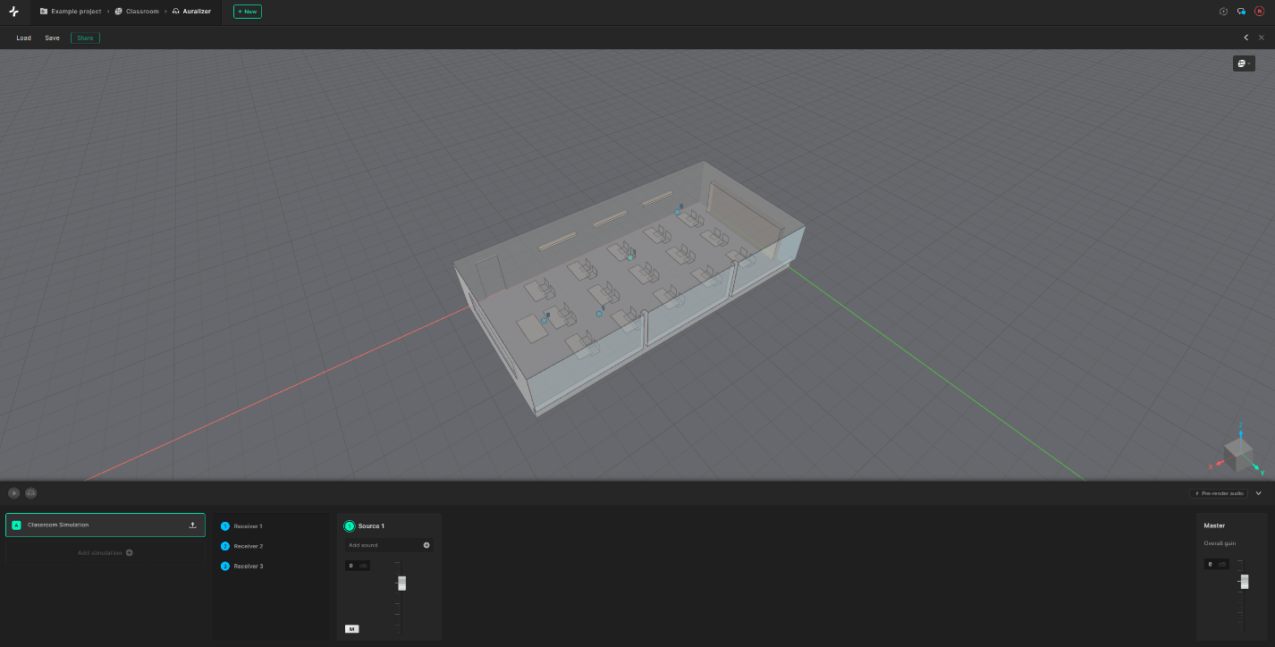
Start by selecting Receiver 1. You will then be able to look around the model at the location of the chosen receiver in a first-person view. You will also be able to see a minimap of the receiver orientation on the bottom right of the screen. This can be expanded or removed if desired. If removed, it can be reinstated via the cube icon in the top right of the screen.
As an advanced functionality, you can upload visual models to the Treble auralizer to enhance the visual realism of the auralization. Similar to the results view, up to six different simulations can be added into comparison within the auralizer.
Click the “Add sound” button under Source 1
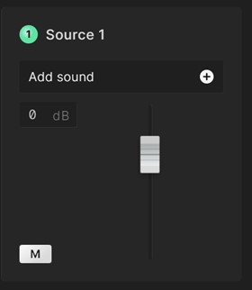
This will open our sound library.
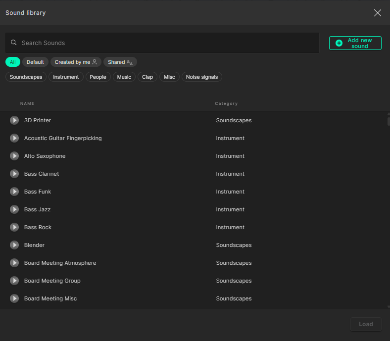
You can preview any sound you’re interested in hearing by using the ’Play’ button next to the audio title. You can then ’Load’ your selected audio in the bottom right corner. We encourage you to try out different sounds and soundscapes. To play a sound click the play button under the model view on the left, to hear the original anechoic recording of the sound signal you can hover over the ’Bypass IR’ icon next to the play icon. You can now also click on the different receivers to see how the acoustics of the space changes based on location.
We always recommend listening to auralizations using headphones as the audio is being played in binaural.
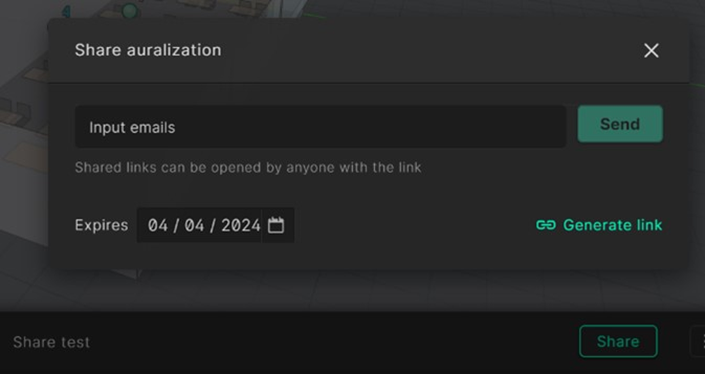
You can also share auralizations with anyone by creating a shareable link which can be sent via email or through a custom url link.
Congratulations! You’ve now finished your first acoustic simulation in Treble. If you are ready to dig deeper into Treble, you can checkout our next guide on how to import your models into Treble.