Setting up a recording device simulation

When setting up a simulation to create a device within Treble, we offer two different interfaces: an easy to use interface, and a more elaborate and customizable one that exposes more parameters. For most cases, we recommend using the simpler interface, but it may sometimes fail for more complex geometries, especially those that may have resonances that must be captured by longer simulations. For such devices, we recommend using the elaborate interface.

When setting up such a simulation, there are a few tunable parameters.

1. Radius of the spherical geometry
   • Here the goal is to set the sphere geometry in such a way that all the energy coming from the source reaches all receivers but does not reflect of the edge and come back to the receivers.
   • The larger the sphere, the more expensive the simulation gets, so it's in your interest to make it as small as possible.
   • The needed size of sphere is frequency dependent as the source width and delay are frequency dependent.
2. Radius of receiver sphere
   • In a sense, the larger, the better. However, with computational interest in mind, we find that a radius of 1 m is generally sufficient.
3. IR length
   • Temporal length of the impulse response to be computed.
   • This ties to the size of domain, receiver sphere and device geometry.
   • A balance between getting all energy to receivers and not getting a reflection back from the exterior surface.
4. Upper frequency of simulation
   • The device will, at maximum, be valid up to this frequency
   • The simulation cost increases rapidly with frequency, so in general it's good to test things at lower frequencies first.
5. Ambisonics order
   • In the simulation, this controls the number of receivers which are distributed around the device
   • From the simulation results you will be able to create devices at an equal or lower order than the simulation accounted for.
   • We have a guide for choosing an appropriate ambisonics order
6. Number of receivers
   • The number of receivers can be tuned, otherwise they follow the ambisonics order.
7. Mesh parameters
   • Meshing parameters, which will not be detailed here, can be tuned for improving the representation of the device geometry in the simulation

These parameters are non-trivial to tune, but the good news is that you do not have to worry about most of them. In the simple interface, these parameters, except for the ambisonics order and upper frequency are tuned for you.

Device creation with simple interface

Using the simple interface, you can set up and run a device creating simulation in just a handful of lines of code. You need to provide the device geometry, or a path to a file containing the geometry, and you need to define where on the device the microphones should be located. Chose the ambisonics order and upper frequency based on the table generated by running this command

treble.free_field.print_ambisonics_order_guideline(sphere_radius=0.20, ambisonics_order=32)

note

The sphere radius should be the maximum receiver distance for all the receivers on your device. Example: you have a soundbar and the outermost microphone sits at y = 0.2m. From the table above the maximum resolvable frequency for 32nd order will be 8734 Hz. If 4300Hz is sufficient frequency range for this device then use ambisonic order 16.

device_geometry = "some_device_file.3dm"

microphone_placements = [treble.Point3d(0.1, 0.0, 0.0), treble.Point3d(-0.1, 0.0, 0.0)]

simulation_definition = project.setup_drtf_simulation(
    simulation_name="some_device_creation", # unique name for simulation definition
    device_geometry=device_geometry,
    freefield_model_name="ff_model_for_some_device", # unique name for new free field model
    device_microphone_placements=microphone_placements,
    frequency=6000, # upper frequency limit for device free field simulation
    ambisonics_order=16 #should be the higher resolvable order for the specified frequency
)

This approach automatically tunes all the previously mentioned parameters automatically in a way is generally optimal for most cases. However, as mentioned previously, it's not guaranteed that it works for devices which cause resonances and late arrivals of energy. From this simulation definition, it can be plotted for closer inspection, added to the project and finally, started.

simulation_definition.plot()

simulation = project.add_simulation(simulation_definition)
simulation.start()

The simulated device can then be used to create a DRTF, to be used for device rendering.

Device creation with advanced interface

Free field model settings

When using the customizable interface, great care must be taken when setting input parameters. The first step is to create the free-field model and tune the optional sphere_geometry_radius, injected_triangle_edge_length, and receiver_sphere_radius_in_m parameters. If not explicitly defined, default values will be used for these parameters. The sphere_geometry_radius depends on the values provided to frequency and device_microphone_placements that are passed to the model creation, and will update automatically if those two values are provided.

# Optional
ff_settings = treble.free_field.FreeFieldModelSettings(frequency=2000, receiver_sphere_radius_in_m=1)

mics = treble.free_field.DeviceMicrophonePlacements(
    list_of_points = [treble.Point3d(0.1, 0, 0), treble.Point3d(-0.1, 0, 0)],
    injected_triangle_edge_length = 8e-3 # Optional
)

ff_m = treble.free_field.add_free_field_model(
    project=project,
    name="ff_model",
    geometry="path_to_device_geometry",
    device_microphone_placements=mics,
    freefield_model_additional_settings=ff_settings
)

At this point, you have a model which can be plotted and analyzed as per usual with other models in the Treble SDK.

Free field simulation definition

Now it's time to create a FreeFieldSimulationDefinition using the already generated model. For that step, you need to tune the number_of_receivers, max_ambisonics_order and some mesher parameters. These all have default value, but as this is presenting the customizable interface, we'll customize them.

# Optional
ff_sim_settings = treble.free_field.FreeFieldSimulationSettings(
    number_of_receivers=1200,
    max_ambisonics_order=16
)

mesher_settings = treble.MesherSettings(simplify_mesh=False)

When looking at / plotting the ff_m model, you can see the layers which microphones have been placed on, and you can tune specific mesher settings for those layers if you belive that to be of interest for you. Normally, it's fine to leave this to the default values though.

# Name of source (microphone) layers
source_layers = ["surface_layer_0", "surface_layer_1"]

local_sizing = [
    treble.LocalMeshSizing(
        layer_name=surface_layers[i], mesh_sizing_m=8e-3, keep_exterior_edges=False
    ) for i in range(len(surface_layers))
]

We now have all the information we need to create the FreeFieldSimulationDefinition

sim_def = treble.free_field.FreeFieldSimulationDefinition(
    name="free_field_simulation",
    free_field_mode=ff_m,
    frequency=6000, # If passed before, has to be the same
    receiver_sphere_radius=1, # If passed before, has to be the same
    simulation_purpose=treble.free_field.FreeFieldSimulationPurpose.device,
    free_field_simulation_settings=ff_sim_settings,
    mesher_settings=mesher_settings,
    local_mesh_sizing=local_sizing
)

Now similarly as in the simple interface, the simulation definition can be plotted, added to the project and run.

sim_def.plot()

simulation = project.add_simulation(sim_def)
simulation.start()

The simulated device can then be used to create a DRTF, to be used for device rendering.

Create a Device from Simulation Results

Upon conclusion of a device creation simulation, it is easy to create the device related transfer function (DRTF) from the results. The first step, is to get the results object.

results = simulation.get_results_object("directory_for_results")

Then, from the results object, there is a method to create a DRTF where we recommend supplying a list of labels for the microphones on the device to make it easy to recognize which is which when looking at the device later on. The order of the labels is the same as the order of the microphones specified when defining the device creating simulation. Now, when creating the DRTF, you will only be able to select an ambisonics order lower or equal to the one defined on the simulation level. We recommend using the (default) option of applying far-field expansion to the simulated data as it more resembles an ideal measurement setup. Applying the far-field expansion is increasingly important as the device geometry gets larger.

Enabling phase linearization allows higher frequencies to be represented more accurately when using low ambisonic orders. It aligns the phase at high frequencies using a single shared delay across directions, reducing spatial phase complexity while preserving the original low-frequency behavior, and with it, key perceptual cues like interaural time differences (ITD). This improves the stability and realism of high-frequency rendering in low-order ambisonic applications.

device_def = results.create_drtf(
    device_name="some_device",
    ambisonics_order=16,
    microphone_labels=["TopRight", "TopLeft"],
    apply_far_field_expansion=True,
    linearize_phase=True
)

This method uses creates a DeviceDefinition object. By then adding the device definition to the device library, the device gets fully created and stored in the device library, resulting in a DeviceObj.

device = tsdk.device_library.add_device(device_def)

The end result can then be analyzed visually.

The created device can be imported in to simulation where there is a spatial receiver. This covered more in depth in our results section.

Analyze Device

We do processing behind the scenes to convert discrete inputs (response from a finite selection of angles) to a continuous representation where we can compute the response from any angle. This is done using a spherical harmonics decomposition of the input data and for a varying degree of complexity of the input data, we need a varying degree of complexity of the spherical harmonics to capture the input. After a device is created and added to the device library, you can use a tool to analyze the device to ensure it captures the intended/expected behavior.

Device analysis widget

Assuming you have a DeviceObj object, you can run this:

device.plot()

If the widget loads with a white background, run the line above, and it should appear correctly. In this section, we'll go through the different parts of the widget and explain what information it provides.

Transfer function

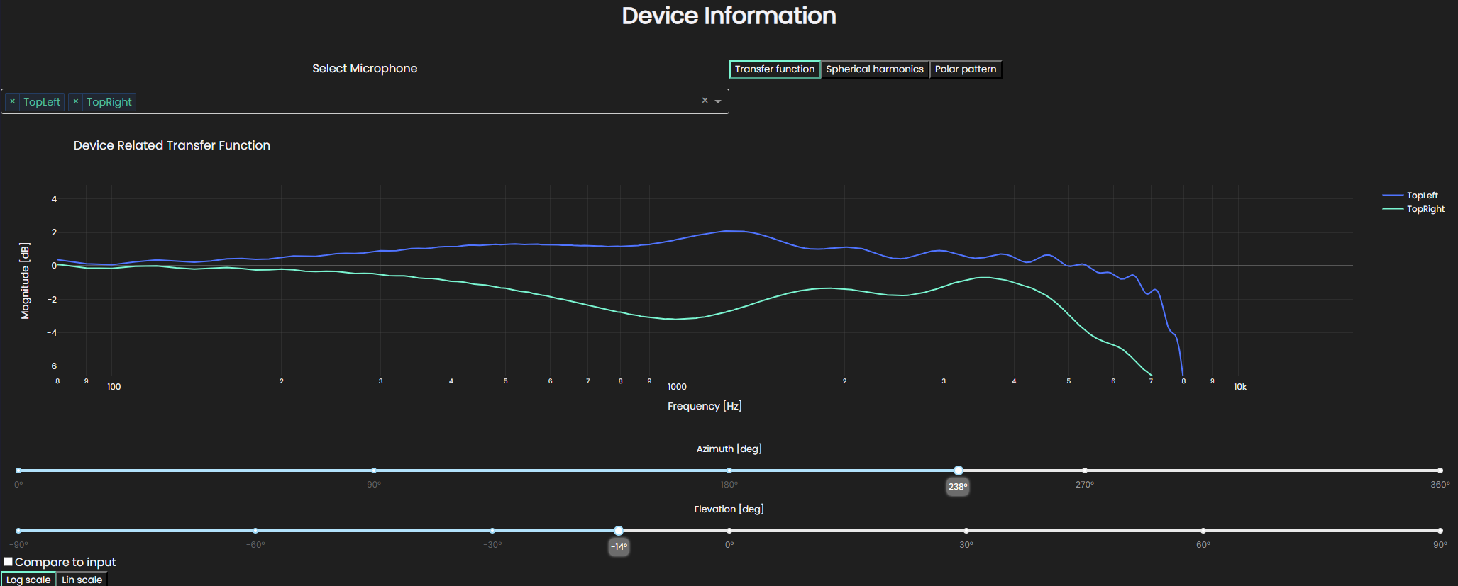
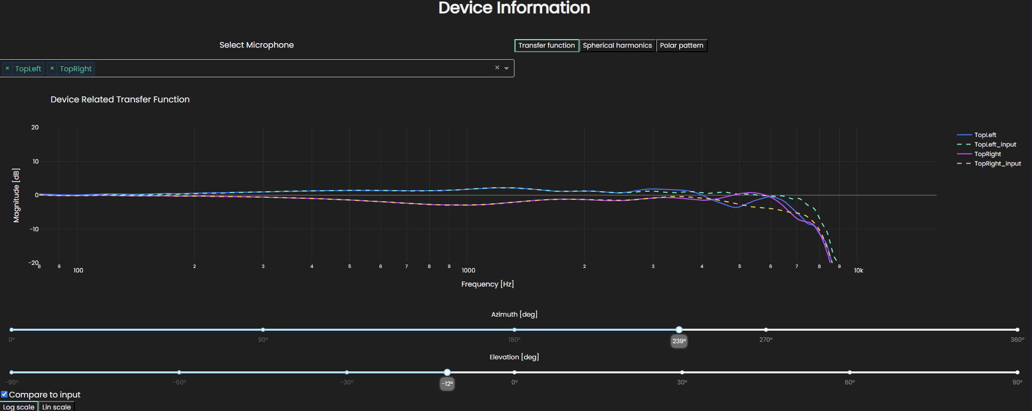
With the Transfer function plotting tool you can look at the response of the device for any direction as a function of frequency with either logarithmic or linear frequency axis. What is displayed is the transfer function computed from the spherical harmonics for the chosen microphones on the device. To investigate, up to which extent the spherical harmonics capture the input data, you can check the Compare to input check mark to plot the input transfer functions in a dashed line. The inputs are only available for selected angles, so this picks the closest angle to what you suggest and plots that. If you opted for applying far-field expansion to the input data, the Compare to input check gets disabled as the comparison becomes somewhat meaningless. We do, however, strongly recommend looking at how well the spherical harmonics captured the input data. Currently, the best way to do so is to create another device from the same input data without applying the far-field expansion and plotting that.

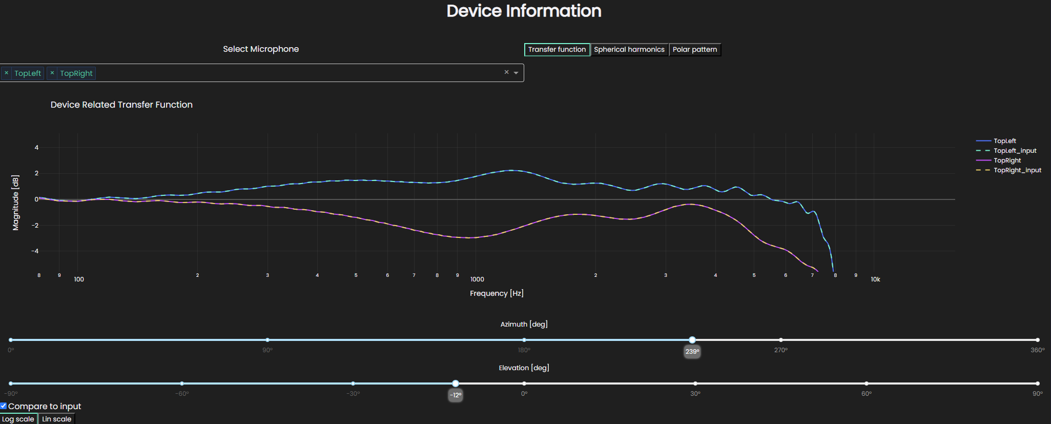
In the displayed case, the spherical harmonics capture the transfer functions perfectly.

Spherical harmonics

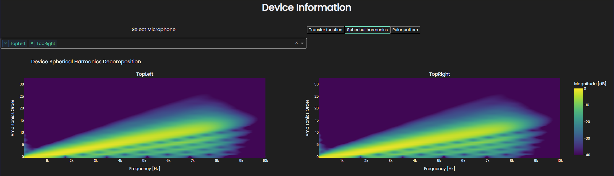
This shows how the energy in the of the microphone directivity is distributed in frequency and ambisonics order. The expected behavior here is that the brightest colors align linearly with a gradient which is controlled by the distance from origin of coordinate system to the microphone. In this particular plot, we also see some fainter colors above the line which relate to the energy which gets diffracted around the device. It can be seen in this plot, where the top of the plot is dark (meaning low energy), that we have a high enough ambisonics order to capture all the energy that we want to capture. This was also reflected in how well the input transfer functions were captured. On the other hand, if we render the same device at a lower ambisonics order, e.g. order 8, we can see that the energy at the top of the plot is still high, so we are not capturing all the energy we would want to.

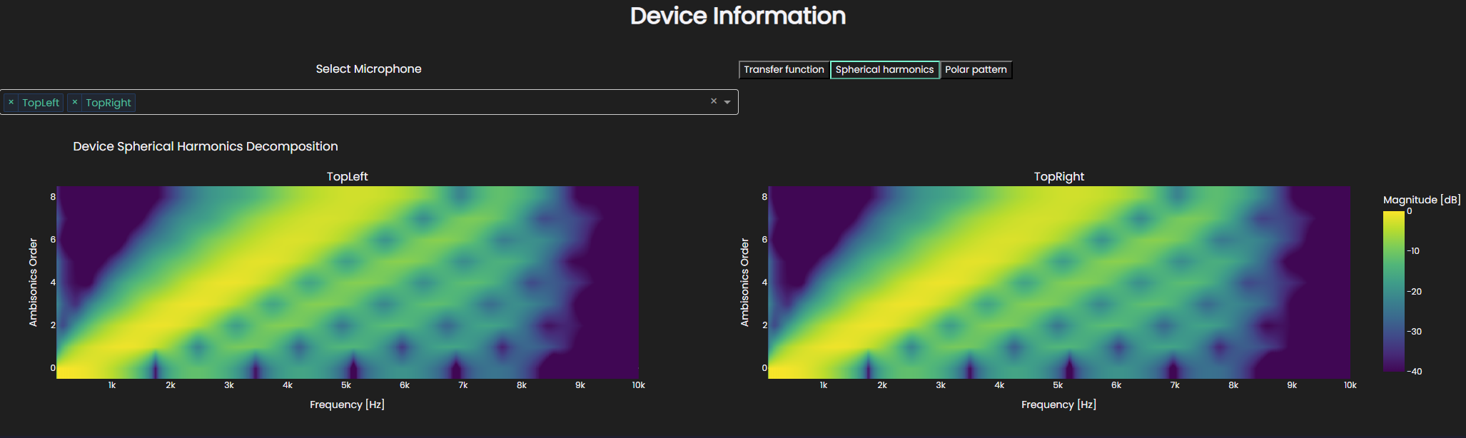
Which we can also see in how the transfer functions are captured, quite well for the lower frequencies, but much worse for the higher ones.

Polar Pattern

The widget also has the option of visualizing the directivity of the microphones in two-dimensional polar pattern for three different planes. The plot is created by computing the response for every angle along the respective plane for a certain frequency. The frequency slider is then used to look at the patterns at different frequencies.

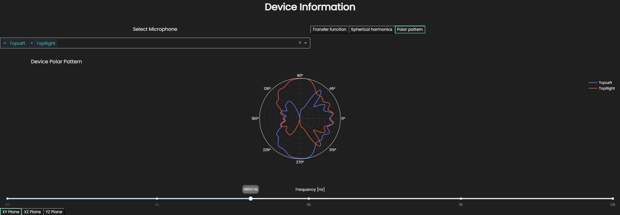
In this particular case, you can see that the microphones have responses which are mirrored around the center.

The created device can be imported in to simulation where there is a spatial receiver. This covered more in depth in our results section(/treble-sdk/results/working-with-data.md)

Create a device from imported DRTFs

When importing a device related transfer function (DRTF) we support the import of raw data from either measurements or simulations. The process is quite simple and just requires a few definitions. Here we provide an example of importing raw DRTF data from an hdf5 file but the file format is irrelevant, it might as well be a sofa, mat, netCDF or even csv or txt. As long as the file contains the right data and you can parse it from the file, you can import the DRTF.

The example file we have is structured like this:

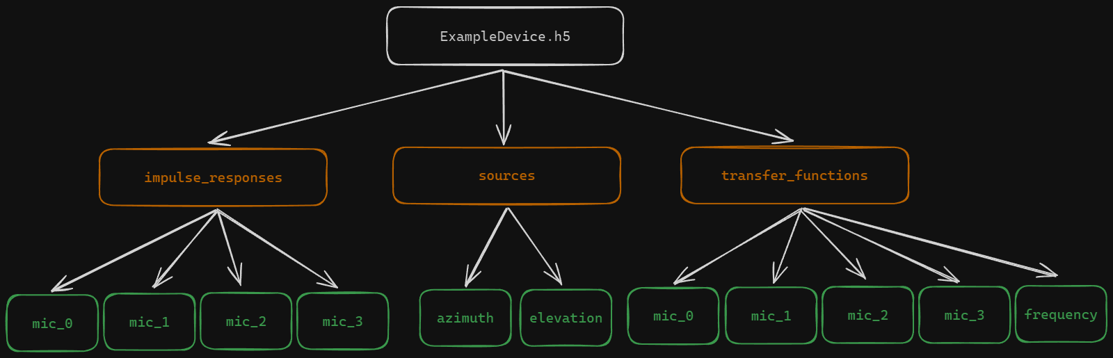
The essential things to define are the source locations on the measurement sphere and either impulse responses or transfer functions of each associated source to a microphone on the device. Each microphone impulse response or transfer function in the file has an array of size number_of_sources x timesteps/frequencies. From a file with such a structure the device can be imported with a simple script showing both option 1 of importing impulse responses and option 2 of importing transfer functions:

import h5py

with h5py.File("ExampleDevice.h5", "r") as f:
    sources = f["sources"]
    sl = treble.DeviceSourceLocations(
        azimuth_deg=sources["azimuth"][:], elevation_deg=sources["elevation"][:]
    )

    dev_microphones = []
    # Optinally you can add labels to microphones to make them more easily recognizable in results
    mic_labels = ["front_center", "back_center", "right", "left"]
    # Here we have two options.
    # Option 1, import impulse responses:
    irs = f["impulse_responses"]
    # Option 2, import transfer functions
    tfs = f["transfer_functions"]
    for n in range(4):
        # Option 1
        ir = treble.DeviceImpulseResponses(
            impulse_responses=irs[f"mic_{n}"][:], sampling_rate=32_000
        )
        dev_microphones.append(
            treble.DeviceMicrophone(
                source_locations=sl, recordings=ir, max_ambisonics_order=16, label=mic_labels[n]
            )
        )

        # Option 2
        tf = treble.DeviceTransferFunctions(
            transfer_functions=tfs[f"mic_{n}"][:],
            frequency_array=tfs["frequency"][:],
            sampling_rate=32_000,
        )
        # dev_microphones.append(treble.DeviceMicrophone(source_locations=sl, recordings=tf, max_ambisonics_order=16))

    device_definition = treble.DeviceDefinition(
        device_microphones=dev_microphones,
        name="DeviceExample",
        description="Device showcase",
    )

device = tsdk.device_library.add_device(device_definition=device_definition)

Now the device has been added to the device library and can be used to render a device response from a spatial impulse response. The device can always be fetched by calling:

device = tsdk.device_library.get_by_name("DeviceExample")