Adding and editing sources

Adding a new source

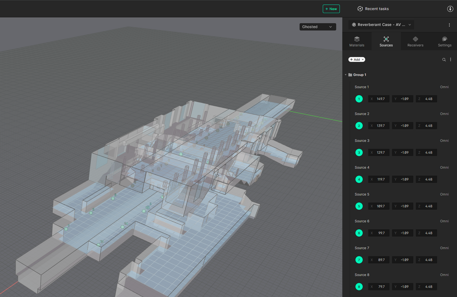
To add a new source, click the Add icon in the Sources field. The first source will appear in the center of the model. Each new source will appear 0.5 m away from the last source, along the x-axis by default. The coordinates can then be edited in the sidepanel. You can have up to 100 sources in a single simulation.

Batch input and offset

Multiple sources can be created in a single operation using the batch creation feature. This is useful when you need to place a number of sources with a regular pattern or spacing. To open it, select the downward-pointing arrow next to the Add split-button. This will open a new pop-up, in which you can both offset a source from a surface and input multiple sources and space them out.

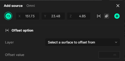
To offset a source from a surface select the offset icon. You can then select a surface to offset from using the dropdown or by clicking on a surface in the viewport. Note that you can offset a single source from multiple surfaces.

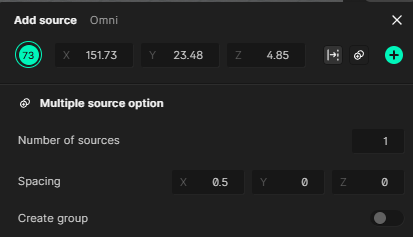
To generate multiple sources select the multiply icon. You can then select how many sources you want to input and space them out along the axis of the coordinate system. Additionally, you can add them all to a single group.

Text file import

Selecting the triple-dot icon next to the Add split-button allows you to import source coordinates via a text file. When uploading via text files, all sources are assumed as omnidirectional, but this can be changed in the sidepanel after the file has been imported. Each line in the file should have three values for the X,Y and Z coordinates respectively. The coordinates should be separated by a comma, for example:

2,2,3
2.5,2.5,3
3,2.5,2.5

The newly created source will appear as a green dot in the 3D view. The source can be selected by clicking the source row in the sidepanel or by clicking the corresponding green dot in the 3D view. The default source definition assigned to new sources is an omnidirectional source.

Make sure that the source is placed inside the model. The minimum distance between a source and a surface depends on both the chosen solver and the transition frequency of the simulation as shown in the following table. Note that the listed frequency denotes the center of the octave band for which the condition applies:

Solver type	Condition	Minimum distance
Geometrical solver	Source to surface	No limit
	Source to receiver	0.5 m
Wave-based solver	Source to surface (125 Hz)	0.5 m
	Source to surface (250 Hz)	0.4 m
	Source to surface (500 Hz)	0.2 m
	Source to surface (1000 Hz)	0.1 m
	Source to surface (2000 Hz)	0.05 m
	Source to receiver	0.5 m

If sources or receivers are placed in an invalid position they will turn red and the simulation cannot be run.

Changing the source type using Treble's source library

To change the source definition for a source, click on the assigned source definition in the upper right corner of a source row (omni by default). This will open the Source definition library to the left of the sidepanel.

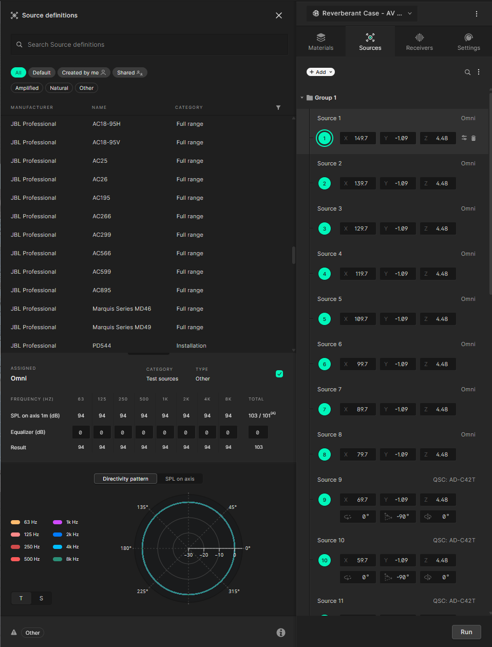
Source definitions are split into three types: Amplified, Natural and Other. Each type contains a unique set of categories.

It is possible to search the library and to filter by the three types as well as by manufacturers or categories.

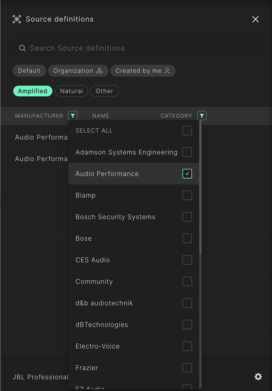
You can also utilize the built-in filters for Default, Organization and Created by me.

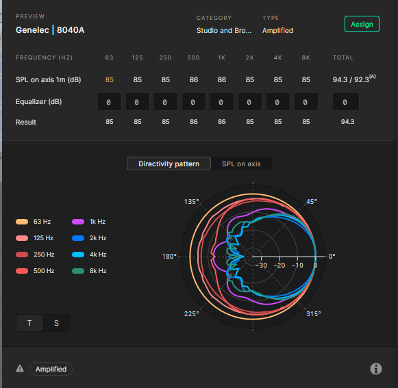
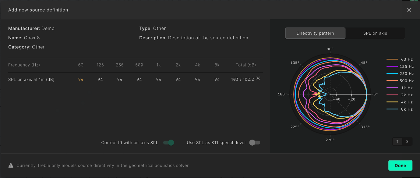
Source definition properties such as directivity pattern and SPL on-axis at 1m are shown at the bottom of the library.

Editing source EQ

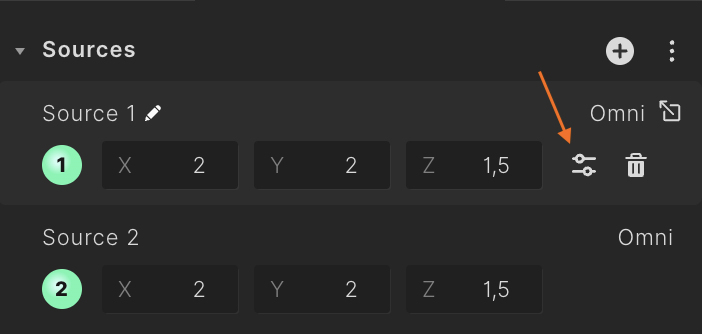
After assigning a source, its properties can be edited by selecting the "settings" icon next to the source coordinates or the name of the source type.

This will open the source definition library. At the bottom of the library, it's possible to edit the EQ. Note that this change will only be applied to the selected source(s) in the current simulation. You can also view the directivity pattern and the SPL on-axis response.

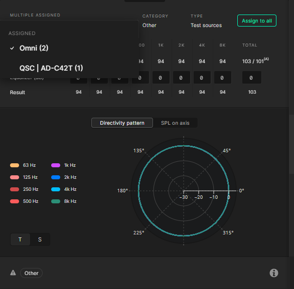
If you have selected sources of different types, you can toggle between them in the dropdown above the frequency response information.

info

The source directivity will only be applied to the GA solver. In the wave-based solver all sources are omnidirectional.

In some cases, the values of the on-axis response in octave bands are colored orange. This is to highlight that this value is extrapolated from the source information and was not a measured value. The full on-axis response can be viewed as a plot on 1/3 octave band resolution.

Directive sources

When a directive source is present (e.g. Speech), the sidepanel will show the orientation as well as the location. When a directive source is selected, a small green arrow will be shown from the controller in the 3D view to help you orient the source.

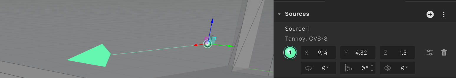
The orientation of a directive source can be edited using the angle input shown in degrees for:

• Azimuth: The azimuth angle will rotate the arrow counterclockwise on the XY plane, starting from the X axis.
• Elevation: The elevation angle starts from 0 and has a range between -90 (-Z) and 90 (Z) degrees.
• Rotation: The counterclockwise rotation around the front facing axis (0 to 360 degrees).

Correct IR with on-axis SPL

The "correct IR with on-axis SPL" toggle can be seen in the Source settings popup. This setting is specifically intended for cases where the source will be used in the auralizer.

When enabled, the impulse response gets corrected with the on-axis SPL levels. It is recommended to enable this for most amplified sources. However, for unamplified sources where the source response is inherently included in the auralized signal, this correction should generally be disabled.

A typical example of this is for simulated speech sources that are assigned a sound file that already contains speech in the auralizer. In such cases, the spectral content originates directly from the sound file itself, and applying an additional correction could distort the intended signal.

Note that the SPL parameter and frequency response plots in the results will always be corrected. When summing sources with corrected and non-corrected IRs the non-corrected ones will also be corrected automatically during the summation process.

Editing sources in a simulation

Once sources have been added to a simulation, you can select, group, and manipulate them using a variety of tools. Click on a source row in the sidepanel to select it. The selected source is highlighted and its details (coordinates, orientation, source definition) become editable. Hold Ctrl (Windows/Linux) or Cmd (Mac) and click additional source rows to add them to the selection, or click an already-selected source to deselect it.

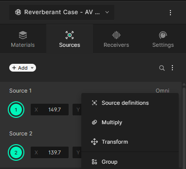
When one or more sources are selected, a floating toolbar appears at the bottom of the 3D viewport. The toolbar shows the number of selected items and provides quick access to the most common actions. You can also right-click on any source row (or on a group header) to open the context menu. The context menu contains the same actions available in the toolbar, plus additional group management options.

Grouping

Groups let you organize related sources together. Grouped sources are displayed under a collapsible group header in the sidepanel and share a color marker in the 3D viewport.

To create a group select two or more sources, then:

• Click Group in the floating toolbar, or
• Right-click and select Group from the context menu, or
• Press Ctrl+G (Windows/Linux) or Cmd+G (Mac).

The selected sources are placed into a new group. The group header appears in the sidepanel at the position of the first grouped source. The group name is editable immediately after creation.

To select a group, click the group header to select all sources in that group.

When a group is selected, you can access group options from the context menu. The Group Options dialog lets you edit:

• Group name: A custom label for the group (e.g. "Stage left speakers").
• Group color: Choose from preset colors, or pick a custom color using the color picker. The chosen color is applied to all source markers in the group in the 3D viewport.

When a full group is selected, choose Ungroup to dissolve the group. All sources become ungrouped individual sources.

When individual sources within a group are selected, choose Remove from group to take them out of the group while keeping the group intact for the remaining members.

When a full group is selected, choose Delete from the context menu. A confirmation dialog will show the group name and the number of sources that will be deleted. Confirming deletes both the group and all its member sources.

Sources and groups can be reordered by dragging them in the sidepanel.

Multiply

The Multiply action creates copies of the selected sources with configurable spacing along the X, Y, and Z axes. This is useful for creating regular grids or lines of sources.

To use multiply, select one or more sources and then click Multiply in the toolbar or context menu:

In the popover, configure:

• Number of copies: How many copies to create per selected source.
• Spacing X / Y / Z: The distance between each copy along each axis (in meters).

A live preview shows the copies in the 3D viewport as you adjust the parameters. Click the Apply button to confirm, or press Enter.

Transform

The Transform action lets you move and rotate selected sources by a specified delta. For sources specifically, it also supports pointing sources toward a receiver.

To use Transform, select one or more sources and click Transform in the toolbar or context menu.

In the popover, configure:

• Move X / Y / Z: The distance to move the sources along each axis (in meters).
• Rotate: The rotation of the source along the horizontal plane (azimuth), vertical plane (elevation), or roll (rotation).
• Point to receiver: Select a receiver from the dropdown to automatically orient all selected sources toward that receiver's position. This overrides the azimuth and elevation values.
• A live preview updates the 3D viewport as you adjust the parameters.

Click the Apply button (checkmark) to confirm, or press Enter. Click the close button (X) or press Escape to cancel and revert.

Offset

The Offset action repositions a single source at a fixed distance from a model surface. This is useful for placing a source at a precise distance from a wall, ceiling, or floor.

To use offset, select a single source, then choose Offset from the toolbar or context menu.

In the popover:

• Layer: Select the surface (layer) you want to offset from. You can browse the model's planar surfaces and click to select one. The surface is highlighted in the viewport when hovered.
• Offset: The distance from the surface to place the source (in meters). The initial value is computed from the source's current position relative to the selected surface. Minimum offset is 0.01 m.

A live preview updates the source position in the 3D viewport, along with an offset arrow indicator. Click the Apply button (checkmark) to confirm, or press Enter. Click the close button (X) to cancel and revert to the original position.

Searching sources

Click the search icon in the Sources header to open the search bar. Type to filter sources by:

• Source label / display name
• Source definition name
• Group name

Sources that don't match the search query are hidden from the sidepanel list.

Uploading a custom source

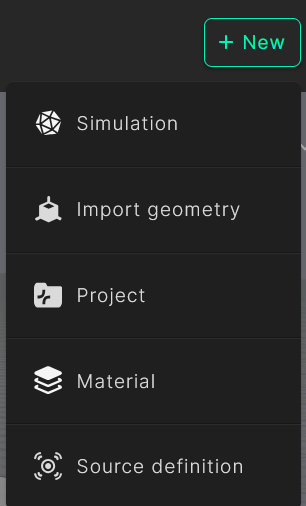
To add a new source definition, click the + New button in the header and in the drop-down menu select Source definition.

The following popup will appear, where you can import a CLF file. Note that only CLF version 2 with the file ending CF2 are accepted. Here you put in a type (Amplified, Natural or Other) and a category based on the type chosen.

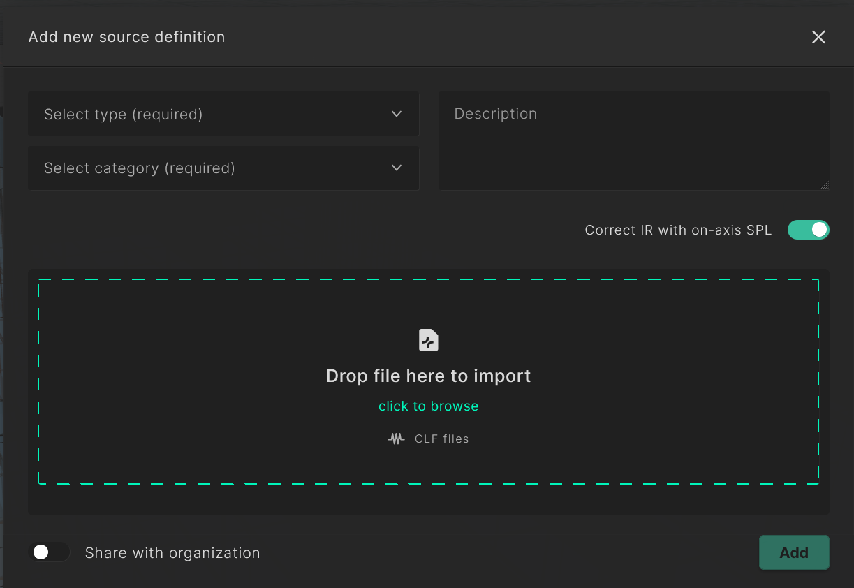
The file undergoes processing, during which the directivity pattern and on-axis response are extracted. Once this process is complete, a source definition details popup will appear. Following this, your new source definition will be accessible in the source definition library.

note

When creating a new source, the toggle "Share with organizations" allows you to add the source to the source library of everyone within your organization, if the organization has a Teams or Enterprise license.