Simulation Settings

Under the "Settings" tab you can modify the simulation settings.

There are two types of solvers available in Treble.

• The wave-based solver - based on discontinuous Galerkin finite element method shortnamed as DGFEM.
• The geometrical acoustics solver - based on a combination of the image source method for early reflection modeling and the ray-tracing method for late reverb modeling.

The geometrical acoustics solver is better suited for high frequencies, whereas the wave-based solver solves the wave equation and gives accurate results at all frequencies. It does, however, take longer time to compute, especially for high frequencies and large rooms. It is therefore a reasonable approach to use a hybrid of the wave-based solver and the geometrical acoustics solver.

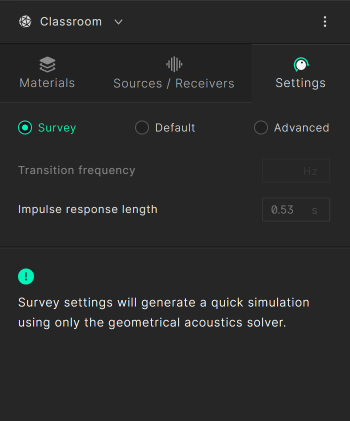
Survey

This option will only use the geometrical acoustics solver as a fast calculation method. Consequently the transition frequency cannot be changed. The impulse response length will be set based on an initial estimate of the reverberation time that depends on the materials assigned.

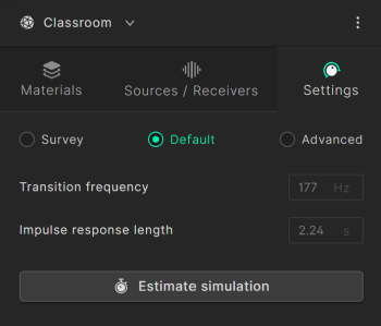
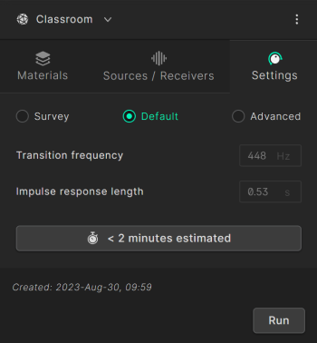
Default

This option will use a hybrid solver, the wave-based solver for low frequencies and the geometrical acoustics solver for high frequencies.

Your model will be analyzed and an optimal transition frequency will be provided automatically. The impulse response below the chosen transition frequency will be calculated using the wave-based solver, whilst the impulse response above the transition frequency will be calculated using the geometrical acoustics solver, and then combined (or hybridized).

Click Estimate simulation to see approx. how long the wave-based solver will take. Clicking this button also generates the volumetric finite element mesh, which the wave solver uses, from the 3D model. If the estimate simulation button is not clicked and instead the run but is clicked directly, the mesh is generated automatically.

Advanced

This option allows the you to modify the given parameters.

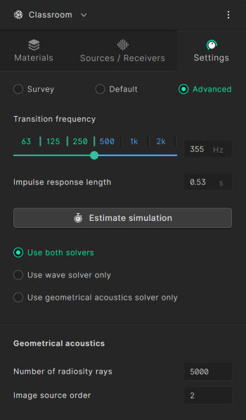
The transition frequency can be modified using the slider or clicking on a frequency band (above the slider). This will be the upper cutoff frequency of the highest octave band that is included in the wave-based simulation. For example if 500Hz octave band needs to be simulated by the wave-based solver, the transition frequency is 710 Hz. The actual transition frequency is shown to the right of the slider. The wave-based solver is accurate but takes longer time. A tip is to set this transition frequency low on the first try to get a feeling for the simulation and meshing time, and then adjust accordingly based on your available resources. Note the meshing and simulation time does not increase linearly with the transition frequency. The simulation time will increase as a fourth order polynomial function of the transition frequency (give a proper warning for a long simulation time with increasing transition freq). The simulation time (the time it takes to run a single simulation) increases linearly with increased impulse response length time (the time duration of the simulated response).

The termination criterion allows for defining one of two different ways of when the simulations should stop. Either when the energy at each receiver has dropped by an energy decay threshold value (defined in dB), or when the simulated IR has reached a certain signal length (defined in s). When the energy decay threshold option is used, an estimated IR length will be shown.

Click Estimate simulation to see approx. how long the wave-based solver will take. Clicking this button also generates the volumetric finite element mesh, which the wave solver uses, from the 3D model. If the estimate simulation button is not clicked and instead the run but is clicked directly, the mesh is generated automatically.

It is possible to use only the w

• Only use wave solver: switches off the geometrical acoustics solver. The simulation will only contain results up to the transition frequency.

• Only use geometrical acoustics solver: This option switches off the wave-based solver so it will be equivalent as Survey option. Simulation results will contain results for the 63-8000 Hz octave bands.

• Image source order: The highest reflection order considered by the image source algorithm for early reflection modeling. Recommended values are 0-3 (higher value implies more accuracy in the geometrical acoustics solver but increases compute time).

• Number of rays: The number of rays used in the geometrical acoustics solver. Larger and more complex geometries typically require more rays for more accurate simulation results, however the ray-tracing part of the GA solver utilizes ray radiosity methods for tracing the energy which does not require a large amount of rays, therefore it is recommended to set the number of rays to a range of 100 to 100'000. The default number is set to 10'000 and can be edited.

Run simulation

A simulation can be started by clicking the Run button.

Then press the Start button in the window that opens up. This sends the job to the Treble cloud service for calculation. The cloud resources allocation usually takes a few seconds. When the simulations have started it is possible to minimize the Run simulation window.

You can create new simulations and edit them freely while waiting for this simulation to finish. Once the simulation is completed it is possible to view the Results or listen to how your space sounds using the Auralizer.

Edit, revert and duplicate a simulation that has been run

For existing simulations, it is possible to either edit a selected simulation and run it again (overriding previous results), or to duplicate it with changed settings.

When changing materials, scattering, sources, receivers or settings of a selected simulation that has been run, a prompt window will appear giving you the option of either Editing the selected simulation or to Duplicate it.

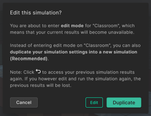
If Edit is selected the Edit mode will start, in which the simulation can be edited as required to run a simulation again. Note that if the simulation is run again after editing, it overrides the previous simulation results. While in edit mode, it is not possible to access previous results or to use the Auralizer.

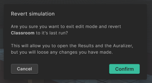
It is possible to exit the Edit mode in case it is not required to run the simulation again. To exit the Edit Mode press the Revert button in the right corner. Reverting will cancel the changes that were made in the Edit mode and go back to the settings of the previously run simulation, making the Results and Auralizer enabled again. A prompt window will appear asking for a confirmation to Revert from the changes that were made.

It is also possible to Duplicate an existing simulation instead of editing it by pressing the Duplicate button when prompted in the Edit window (see Edit Mode Picture above). This creates a new simulation based on the selected simulation, adding " - Copy" to the end of its name. This Duplicate simulation will also include the change made in Edit Mode.

Example: You click to add a new source, and then press Duplicate. Then the new source will appear in the new duplicated simulation.

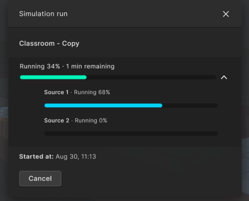
Run status

To inspect the simulation progress click on Show run status.

This is the Simulation run view. The process for each source can be shown by opening the drop-down.

Video-guide

Simulation settings in Treble: