Boundary velocity submodels
Boundary-velocity submodels let you simulate physical sound sources by applying a normal velocity condition to a specified region of the source geometry. This accurately captures source directivity effects caused by baffle diffraction.
Treble generates boundary velocity submodels from a wave-based free-field simulation and saves them as reusable library objects, so teams across your organization can apply the same validated source model in multiple projects. See Create a boundary velocity submodel.
To separate a source into its passive and active parts, Treble uses the same geometry layer-based workflow as in regular room simulations.
Boundary velocity submodels behave differently depending on the solver:
- Wave-based solver: Treble injects the full source geometry into the room mesh and applies a velocity condition to the membrane.
- Geometrical acoustics solver: Treble fits a directive point source to the simulated radiation pattern.
Boundary velocity submodels are therefore compatible with wave-based, geometrical, and hybrid simulations. See a validation study for details.
Boundary velocity submodels are calibrated to produce a flat on-axis frequency response at 1 meter in anechoic conditions, up to their upper frequency limit.
Basic examples
Generate loudspeaker geometry
Pass cabinet dimensions and membrane parameters to generate a box-shaped loudspeaker geometry:
# Create loudspeaker shaped geometry component
loudspeaker = treble.GeometryComponentGenerator.create_loudspeaker(
    width=0.15,
    depth=0.15,
    height=0.15,
    membrane_diameter=0.05,
    membrane_center_height=0.075,
)
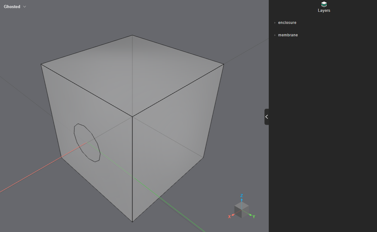
Verify the result:
loudspeaker.plot()
Import loudspeaker geometry from CAD
Upload your CAD file as a model. Supported formats are .3dm, .obj, and .dxf. See Importing geometry for details.
# Import loudspeaker geometry component and wait for geometry processing
imported_loudspeaker = project.add_model(
    model_name="<model_name>",
    model_file_path="<model_file_path>"
)
imported_loudspeaker.wait_for_model_processing()
wait_for_model_processing() blocks until the geometry is ready for use.
imported_loudspeaker.plot()
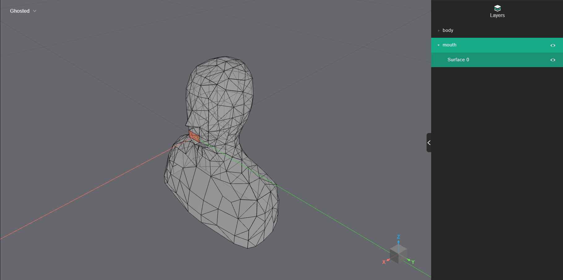
Make sure your radiating surface is a separate, unique layer in the geometry. Apply fully reflective materials to the rest of the surfaces for best simulation results.
Create a boundary velocity submodel
Wrap source geometry in a spherical enclosure
Use the free_field module to create free-field models. It wraps your source
geometry in a spherical domain:
from treble_tsdk import free_field as ff

# Generate and add free-field model to project
free_field_model = ff.model.add_free_field_model(
    project=project,
    name="<model_name>",
    geometry=loudspeaker, # your source geometry
)
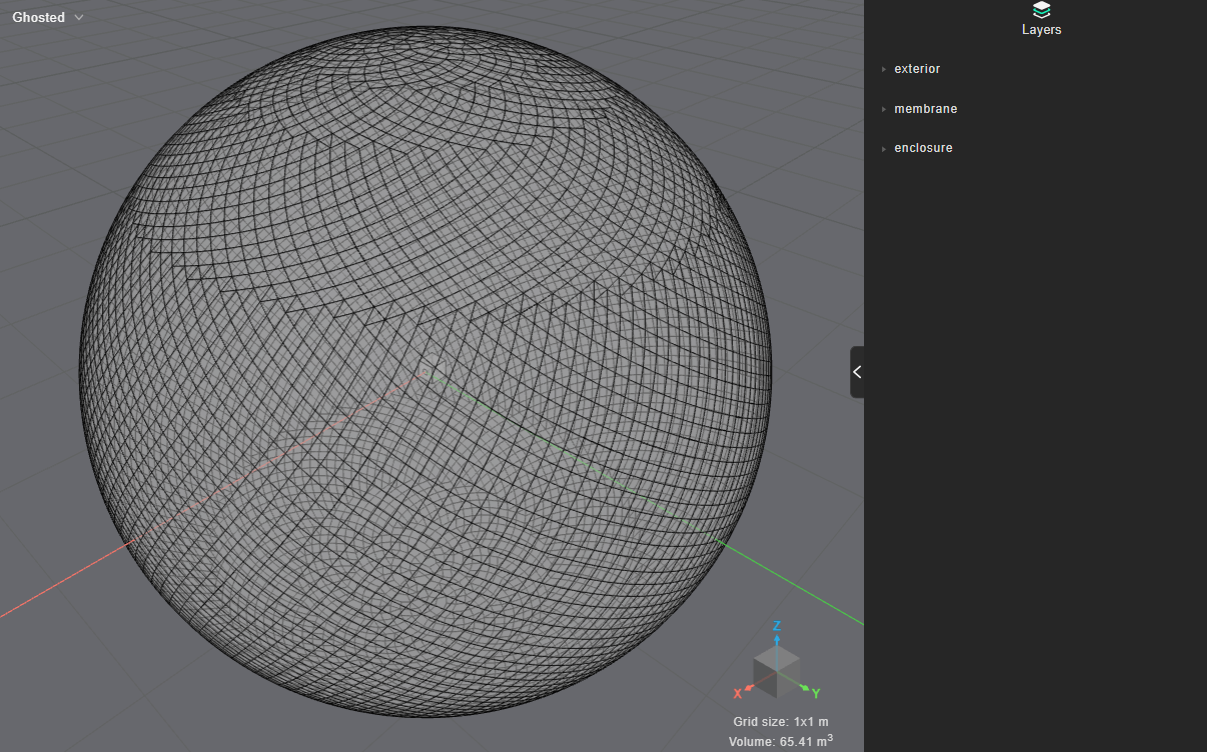
Treble sizes the domain automatically around the device geometry.
free_field_model.plot()
Define free-field simulation
Define a FreeFieldSimulationDefinition up to your preferred frequency,
passing the active layer name as the source_input parameter.
free_field_simulation_definition = ff.FreeFieldSimulationDefinition(
    name="<simulation_name>",
    free_field_model=free_field_model,
    frequency=6000,    # determines mesh sizing and valid frequency range
    source_input="<source_layer_name>", # layer name of the active surface
)
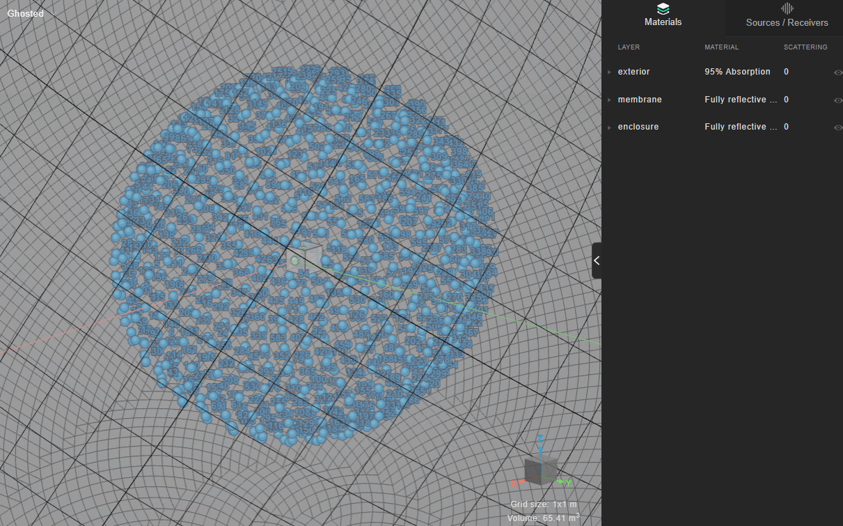
Plot the setup to verify your free-field simulation before submitting. Make sure the sphere receivers and domain fully encapsulate your speaker's geometry.
free_field_simulation_definition.plot()
Add the simulation to your project to trigger meshing in the cloud:
# In case the simulation already exists (from previous run)
free_field_simulation = project.get_simulation_by_name(free_field_simulation_definition.name)

if not free_field_simulation:
    free_field_simulation = project.add_simulation(free_field_simulation_definition)
To get a time and cost estimate for running the free-field simulation:
from treble_tsdk import display_data as dd

# wait for estimate and display graphical element
dd.display(free_field_simulation.wait_for_estimate())
Run simulation
When you're ready, start the simulation:
free_field_simulation.start()
Get results
Once the simulation has completed, fetch the results:
results = free_field_simulation.get_results_object(free_field_simulation.id)
Call results.plot_directivity_balloon(frequency) at a few frequencies to verify the radiation pattern meets your expectations before storing it as a submodel.
Add sound source to your organization's library
Once the results look correct, store it as a submodel:
submodel = results.create_boundary_velocity_submodel(
    source_name="<submodel_name>",
    source_description="<description>",
)
Your organization will now have access to the submodel via the submodel library. See how to access the library.
Access the boundary velocity submodel library
Retrieve a submodel by name or ID for exact lookups, list all available sources, or search by substring:
# get by name or id
tsdk.boundary_velocity_submodel_library.get_by_name('<submodel_name>')
tsdk.boundary_velocity_submodel_library.get_by_id('<submodel_id>')

# lists all sources
tsdk.boundary_velocity_submodel_library.get_sources()

# search by substring
tsdk.boundary_velocity_submodel_library.query('<search_term>')
Rename a submodel
Rename a submodel:
tsdk.boundary_velocity_submodel_library.rename_submodel(submodel, new_name='<new_name>')
Renaming a submodel won't break simulations that reference it. However,
scripts or notebooks that retrieve the submodel using get_by_name must be
updated to use the new name.
To avoid issues caused by renaming, prefer retrieving submodels with get_by_id.
Delete a submodel
Deleting a submodel removes it from your organization's library permanently:
tsdk.boundary_velocity_submodel_library.delete(submodel)
Use boundary velocity submodel in simulations
Retrieve the submodel and construct a Source object for use in simulations:
submodel = tsdk.boundary_velocity_submodel_library.get_by_name("<submodel_name>")

source = treble.Source.make_boundary_velocity_submodel(
    location=treble.Point3d(1, 2, 3),
    orientation=treble.Rotation(azimuth=30),
    boundary_velocity_submodel=submodel,
    label="<source_label>",
)
Multiple submodels can coexist as sources in the same simulation.
Near-field behavior is accurate as long as the membrane isn't intersected by the room geometry. Placing the speaker in a corner or close to a wall affects its radiation pattern, as it would for a physical source.
Plot source far-field directivity
Plot the radiation pattern across the simulated frequency range:
submodel.plot()
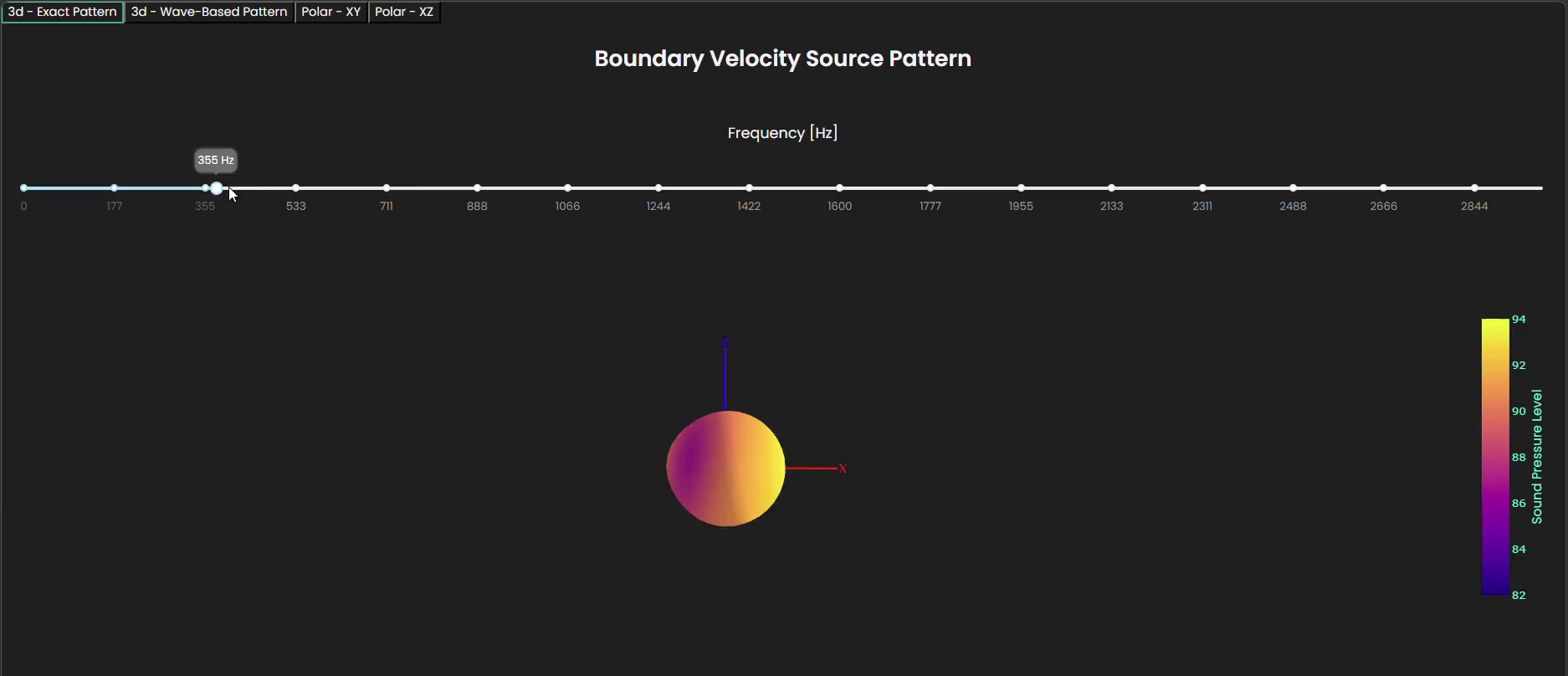
The frequency slider steps through the simulated range. Three tabs let you switch between views:
- 3d - Exact Pattern: the directivity balloon measured from the free-field receivers, colored by SPL
- Polar - XY: 2D polar cut in the horizontal plane
- Polar - XZ: 2D polar cut in the vertical plane
A 3d - Wave-Based Pattern tab also appears in the plot but is not supported for boundary velocity submodels and will not display data. It will be removed in a future release.
Plot source geometry
Plot the device geometry, with layer information:
submodel.plot_geometry()
Advanced examples
Position and orient geometry from CAD
The orientation of the source geometry in the free-field simulation defines the reference orientation of the submodel's directivity pattern. If your CAD file places the loudspeaker facing the wrong axis, or at the wrong height, apply a Transform3d before running the free-field simulation to correct it.
To control placement, wrap the model in a GeometryComponent with a Transform3d:
# Translate the source 0.5 m along the Z axis (e.g., lift it off the ground)
transform = treble.Transform3d(
    translation=treble.Vector3d(0.0, 0.0, 0.5),
    # Rotate 45 degrees around the vertical axis (azimuth), leaving elevation and bank at 0
    rotation=treble.Rotation(azimuth=45),
)

# Wrap the model in a component so the transform is applied before the free-field simulation
loudspeaker = treble.GeometryComponentGenerator.create_component_from_model(
    model=loudspeaker,
    component_name="<component_name>",
    transform=transform,
)
This translates the geometry 0.5 m along the Z axis and rotates it 45 degrees around the vertical axis. Pass the result to add_free_field_model in place of the raw model.
Import specific layers from a CAD model
To control placement, wrap the model in a GeometryComponent using layer_names to restrict the component to specific layers:
loudspeaker = treble.GeometryComponentGenerator.create_component_from_model(
    model=loudspeaker_in_complex_surroundings,
    component_name="<component_name>",
    layer_names=["membrane", "baffle"],
)
This also works when a single model contains multiple speaker variants.
Orient a source toward a receiver
Instead of computing a rotation manually, pass a Point3d or Receiver as the orientation and the source will be oriented toward that target automatically:
receiver = treble.Receiver.make_mono(location=treble.Point3d(3, 0, 1.2), label="listener")

source = treble.Source.make_boundary_velocity_submodel(
    location=treble.Point3d(0, 0, 1.0),
    boundary_velocity_submodel=submodel,
    label="<source_label>",
    orientation=receiver,
)
An existing source can be re-oriented in the same way with source.look_at(receiver).
Create directive point source from free-field results
If near-field accuracy and geometry injection aren't needed, create a directional point source from the same results object instead:
directivity = free_field_results.create_source_directivity(name="<directivity_name>")
Treble stores this in tsdk.source_directivity_library. It behaves like any other directional source and works with all solver types.