Acoustic parameters

Acoustic parameters summarize key properties of an impulse response. They are fundamentally defined for mono impulse responses; when working with spatial impulse responses, they are derived from the omni channel. In Treble, they’re pre-computed for each source-receiver pair in a Results object obtained from a completed simulation. You can retrieve, inspect, and plot them to compare acoustic conditions and validate a space’s acoustic behavior. See Results for details on obtaining a results object. Available parameters are listed in the Parameter reference section at the end of this page.

Basic examples

Retrieving acoustic parameters

Get standard acoustic parameters (T20, T30, EDT, C50, C80, D50, etc.) across source-receiver pairs via results.get_acoustic_parameters():

# Get acoustic parameters for a specific source-receiver pair
acoustic_parameters = results.get_acoustic_parameters(
    source="<source_label>",
    receiver="<receiver_label>",
)

Accessing parameters as lists

Access the center frequencies and clarity values for each band directly from the acoustic_parameters object:

acoustic_parameters = results.get_acoustic_parameters(
    source="<source_label>",
    receiver="<receiver_label>",
)

c80 = acoustic_parameters.c80
t20 = acoustic_parameters.t20

List supported parameters

List all available parameters:

acoustic_parameters = results.get_acoustic_parameters(
    source="<source_label>",
    receiver="<receiver_label>",
)

acoustic_parameters.supported_parameters()

Center bands

Get a list of the standard full-octave band frequencies from 63 Hz to 8000 Hz. These band labels are used to index per-octave-band parameters.

acoustic_parameters = results.get_acoustic_parameters(
    source="<source_label>",
    receiver="<receiver_label>",
)

acoustic_parameters.center_bands
# Returns: ['63', '125', '250', '500', '1000', '2000', '4000', '8000']

Plot overview

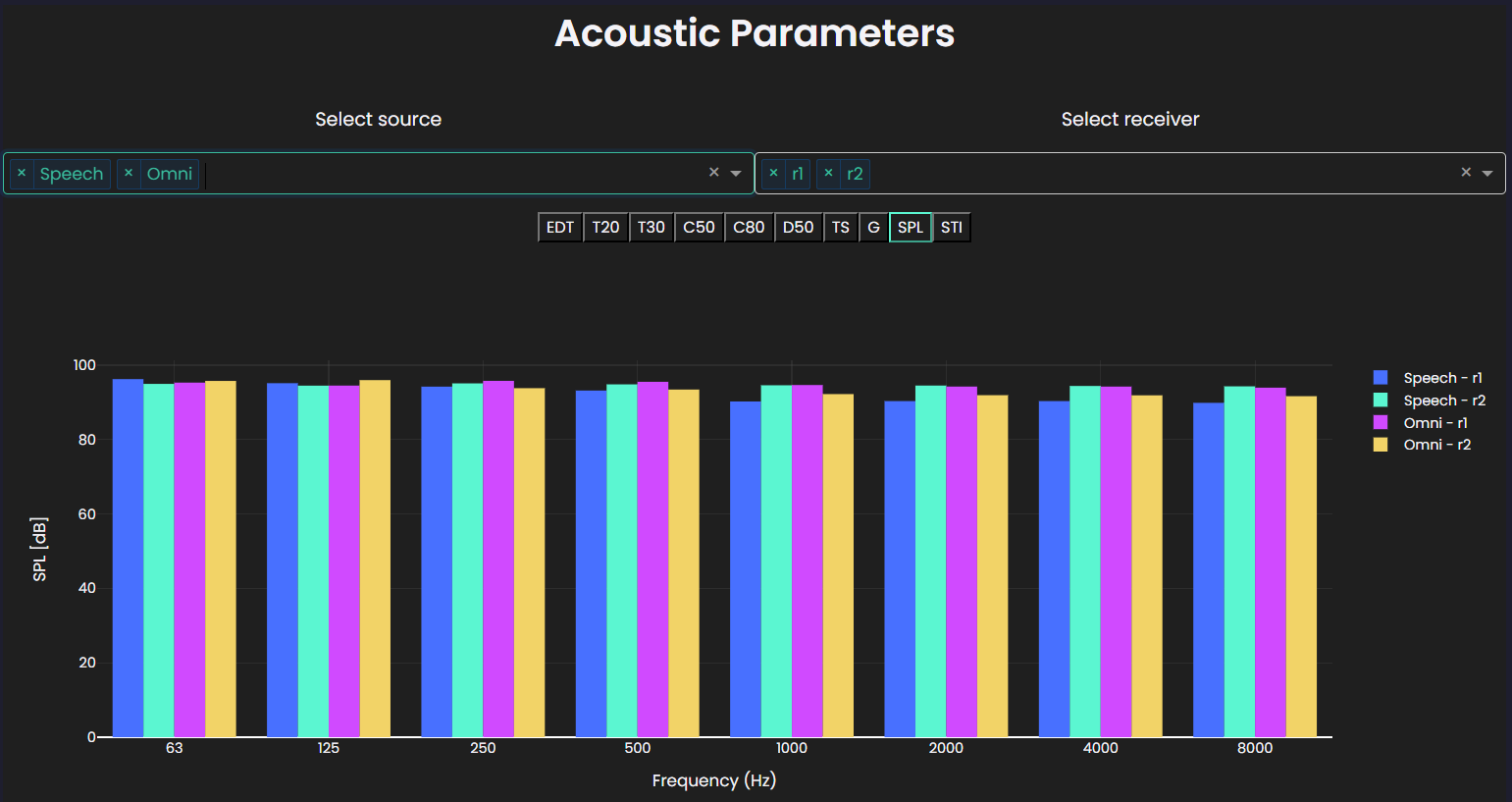
Use the overview widget to compare parameters across all pairs:

# Display interactive overview from results object
results.plot_acoustic_parameters()

Plot for a source-receiver pair

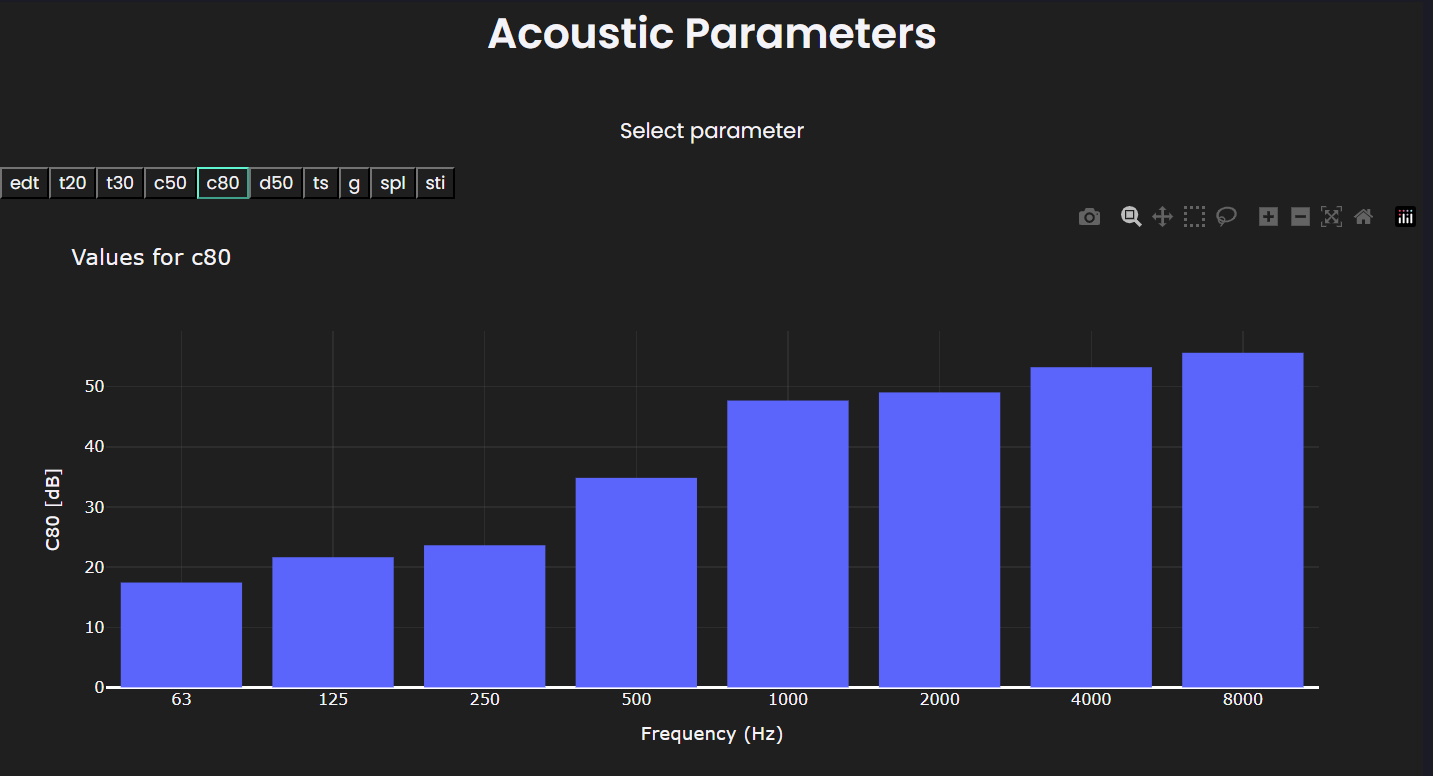
Use the source-receiver pair plot to inspect acoustic parameters for a single pair:

acoustic_parameters = results.get_acoustic_parameters(
    source="<source_label>",
    receiver="<receiver_label>",
)

# Display interactive acoustic parameter widget
acoustic_parameters.plot()

Advanced examples

MTF visualization

The modulation transfer function (MTF) describes how well the acoustic channel preserves amplitude modulation across the frequency bands of an impulse response.

The returned MTF values are flattened. They can be reshaped into eight center bands by 14 modulation frequencies:

import numpy as np
from matplotlib import pyplot as plt

# The MTF values are returned as a list.
# Reshape them into an array with:
# - 8 rows: acoustic center frequency bands
# - 14 columns: modulation frequencies
mtf = np.array(acoustic_parameters.mtf).reshape(8, 14)

# Modulation frequencies used in the MTF calculation, in Hz.
modulation_frequencies = [
    0.63,
    0.8,
    1.0,
    1.25,
    1.6,
    2.0,
    2.5,
    3.15,
    4.0,
    5.0,
    6.3,
    8.0,
    10.0,
    12.5,
]

# Acoustic center frequency bands used for the analysis.
center_bands = acoustic_parameters.center_bands

Each line represents one modulation frequency, plotted across the center frequency bands. Values closer to 1 indicate stronger modulation preservation. Visualize the MTF using the following code:

# Create the figure and axis for the heatmap.
fig, ax = plt.subplots()

# Display the MTF data as a heatmap.
im = ax.imshow(mtf, aspect="auto", origin="lower", cmap="binary")

# Configure the x-axis to show modulation frequency labels.
ax.set(
    xticks=range(len(modulation_frequencies)),
    xticklabels=modulation_frequencies,
    xlabel="Modulation frequency",
)

# Configure the y-axis to show center band labels.
ax.set(
    yticks=range(len(acoustic_parameters.center_bands)),
    yticklabels=acoustic_parameters.center_bands,
    ylabel="Center band",
)

# Add a colorbar to indicate the amplitude represented by the heatmap values.
cbar = fig.colorbar(im, ax=ax)
cbar.set_label("Amplitude")

plt.show()

The resulting heatmap is shown in the following figure.

Missing values

Troubleshooting missing values

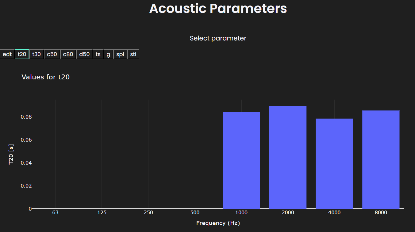
nan values indicate that the computation for a given acoustic parameter couldn't be completed.

This most commonly happens when the impulse response is too short or doesn't contain enough usable information for the requested parameter. For example, when estimating reverberation time, the energy decay curve (EDC) must have sufficient dynamic range. If the EDC doesn't provide enough decay range for a reliable RT estimate in a given octave band, the result will be nan.

acoustic_parameters.t20

[
    nan,
    nan,
    nan,
    nan,
    0.08432203424025161,
    0.08921982691349009,
    0.07852800927916843,
    0.08557646801787988,
]

Plots omit parameters with nan values, so they appear as missing data points.

Parameter reference

The following tables list all acoustic parameters pre-computed by the SDK. For mathematical definitions, see the technical reference pages linked in each row.

Time-based parameters (seconds)

Parameter	Description	Values
`edt`	Early decay time, describing the initial rate of sound decay (read more)	Per octave band (eight values, 63 Hz to 8000 Hz)
`t20`	Reverberation time estimated from a 20 dB decay range (read more)	Per octave band (eight values, 63 Hz to 8000 Hz)
`t30`	Reverberation time estimated from a 30 dB decay range (read more)	Per octave band (eight values, 63 Hz to 8000 Hz)
`ts`	Center time, describing the temporal balance of the impulse response (read more)	Per octave band (eight values, 63 Hz to 8000 Hz)

dB values

Parameter	Description	Values
`c50`	Clarity for speech, comparing early to late arriving sound energy (read more)	Per octave band (eight values, 63 Hz to 8000 Hz)
`c80`	Clarity for music, comparing early to late arriving sound energy (read more)	Per octave band (eight values, 63 Hz to 8000 Hz)
`g`	Sound strength, describing the level contribution from the room (read more)	Per octave band (eight values, 63 Hz to 8000 Hz)
`spl`	Sound pressure level (read more)	Per octave band (eight values, 63 Hz to 8000 Hz)
`spl_a`	A-weighted sound pressure level (read more)	Broadband (one value)
`spl_c`	C-weighted sound pressure level (read more)	Broadband (one value)
`spl_z`	Z-weighted, or unweighted, sound pressure level (read more)	Broadband (one value)
`l_j`	Level-related STI intermediate value per band (read more)	Per octave band (eight values, 63 Hz to 8000 Hz)
`l_j_avg`	Average level-related STI intermediate value (read more)	Broadband (one value)

Ratios (0 to 1)

Parameter	Description	Values
`d50`	Definition, the ratio of early sound energy to total sound energy (read more)	Per octave band (eight values, 63 Hz to 8000 Hz)
`sti`	Speech transmission index (read more)	12 values (one per NC15 to NC70 noise level)
`sti_using_spl`	Speech transmission index computed using SPL-related data (read more)	12 values (one per NC15 to NC70 noise level)
`mtf`	Modulation transfer function, describing modulation preservation across bands (read more)	eight bands × 14 modulation frequencies (112 values)
`j_lf`	Level-dependent auditory masking correction used in STI-related calculations (read more)	Per octave band (eight values, 63 Hz to 8000 Hz)

Basic examples​

Retrieving acoustic parameters​

Accessing parameters as lists​

List supported parameters​

Center bands​

Plot overview​

Plot for a source-receiver pair​

Advanced examples​

MTF visualization​

Missing values​

Troubleshooting missing values​

Parameter reference​